Computer Graphics CS

Learning Outcomes

On completion of this lesson you will know to:

• use tringonometrical functions to calculate coordinates of shapes
• translate entire shapes into the first quadrant so that they can be mapped onto a two dimensional list

Introduction

So far in our lessons we have managed to map the Cartesian plane onto two dimensional lists. This was because we deliberately kept the coordinates of our shapes in the first quadrant of the plane. In other words all of our x and y values were either zero or positive numbers.

In this lesson we plan to rotate a rectangular shape through 180 degrees. This means that we shall making extensive use of trigonometrical functions. Complexity of calculation and of programming code will be reduced if we use (0, 0) as the centre of the rotation. This, however, means that most of our points will be outside of the first quadrant. Therefore prior to mapping our coordinates onto a list we must first translate them into the first quadrant.

Using the origin as point of reference

Below we have an example of using the origin as our starting point

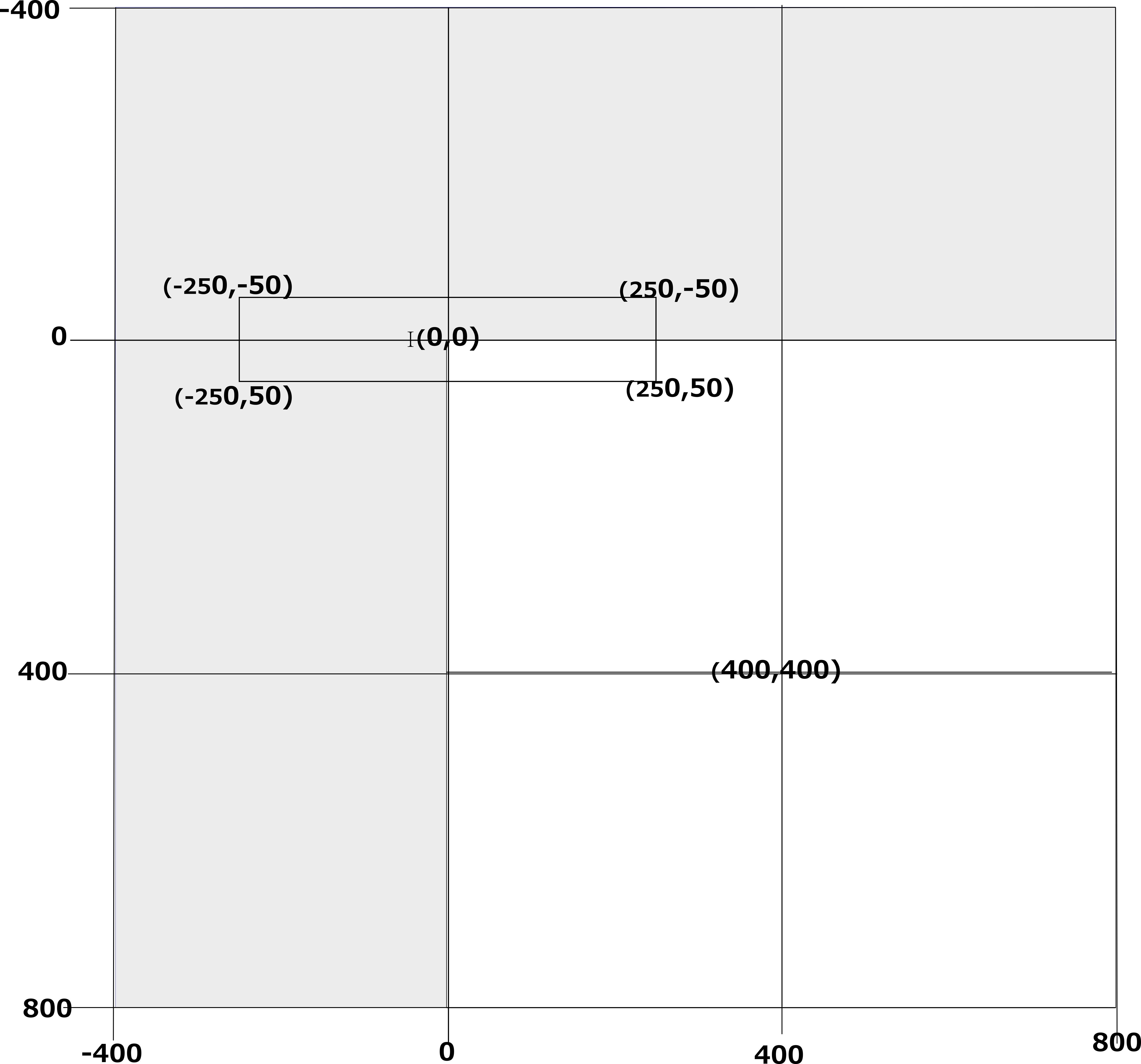
Fig 1 below shows how we start off.

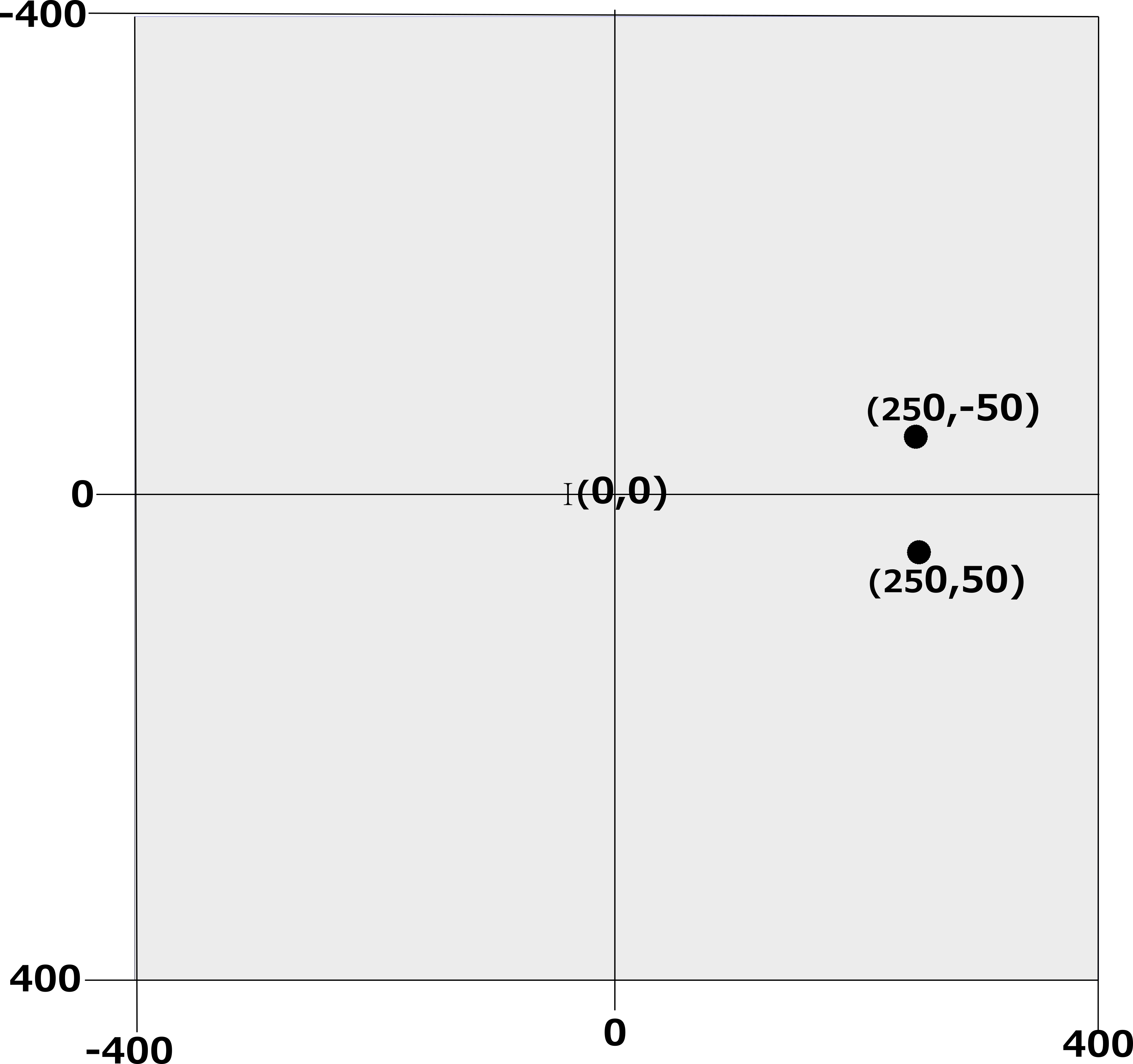
First of all notice the difference between our Cartesion plane here and what is used in conventional mathematics: the y axis increases from top to botton. This is the reverse of coordinate geometry where the y axis increases from bottom to top.

Here we start of with an almost empty plane. We only have two points, (250, 50) and (250, -50) as shown. To make our shapes symmetrical around the origin we draw an imaginary line from each of the points to the origin and extend it the same distance outwards as shown in Fig 2 below.

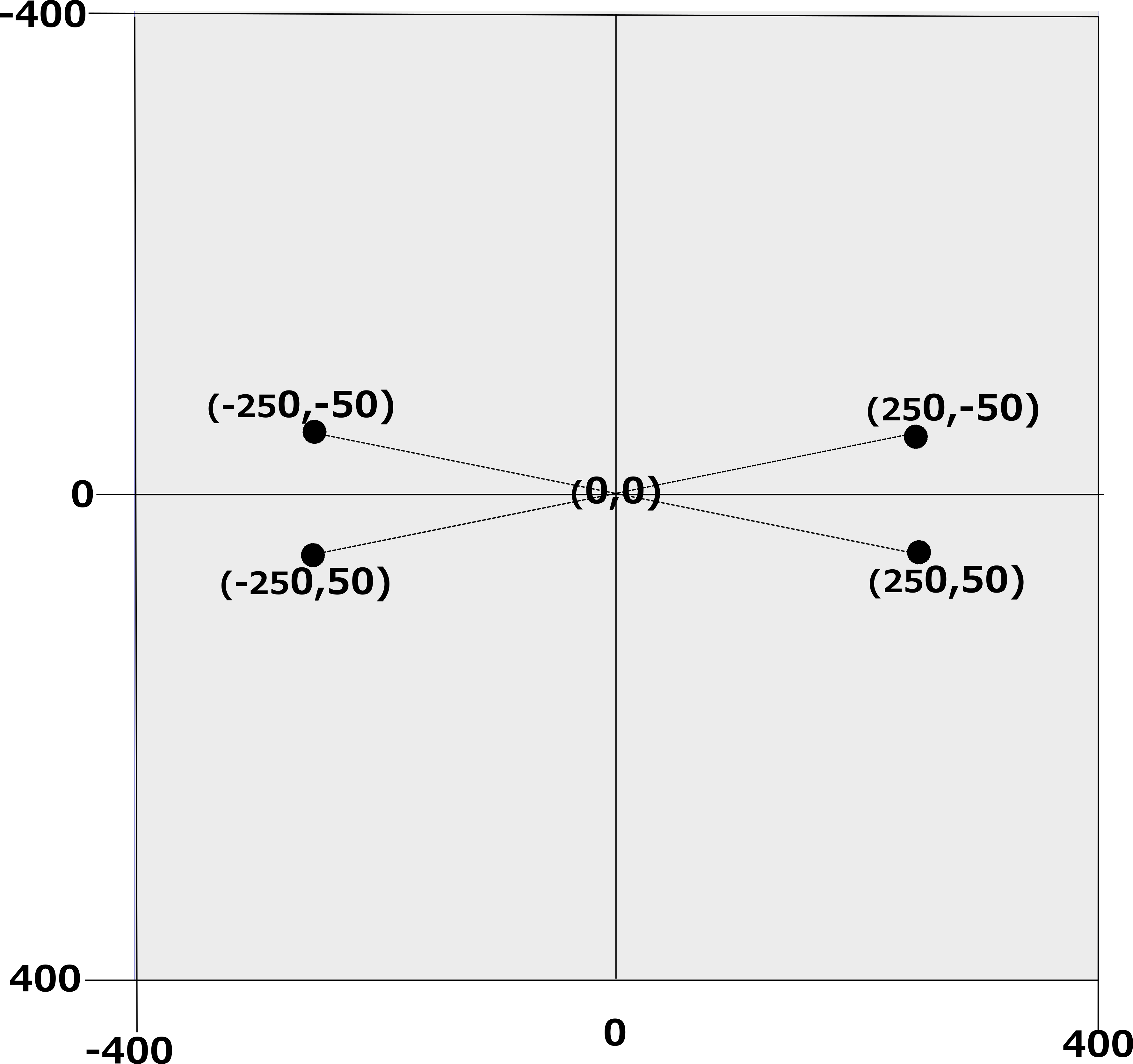
By extending our original two points through the origin we get two more points which make up the four vertices of our quadrialteral. Notice how easy it is to calculate the coordinates of the new points: you simple multiply the coordinates of the original point by -1.

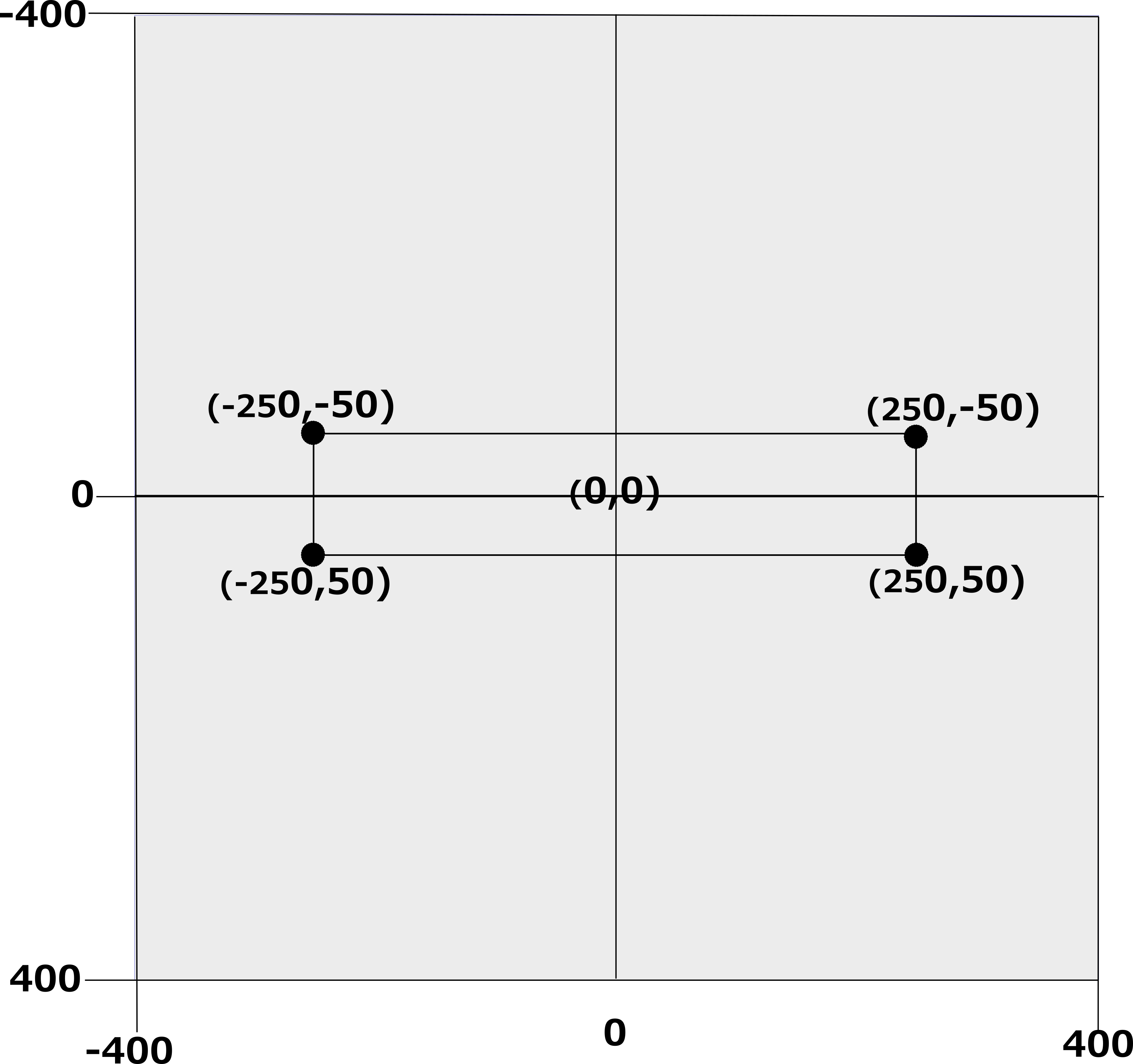
This shows the outline of the shape that we will be drawing. We shall not be actually drawing the shape by tracing its outline: instead we shall filling it in by comparing areas of triangles, just as we did in the previous lesson.

As stated above, centering our shape on the origin it will make our calculations and our codeing easier. However at any time only a quarter of the the area will be in the first quadrant and thus fitting into our two dimensional list will not work.

We have to move our shape away from the origin.

Moving from the origin

For displaying the shape outlined in Fig 3 above we have to extend our plane as far as (800, 800). This is shown in Fig 4 below.

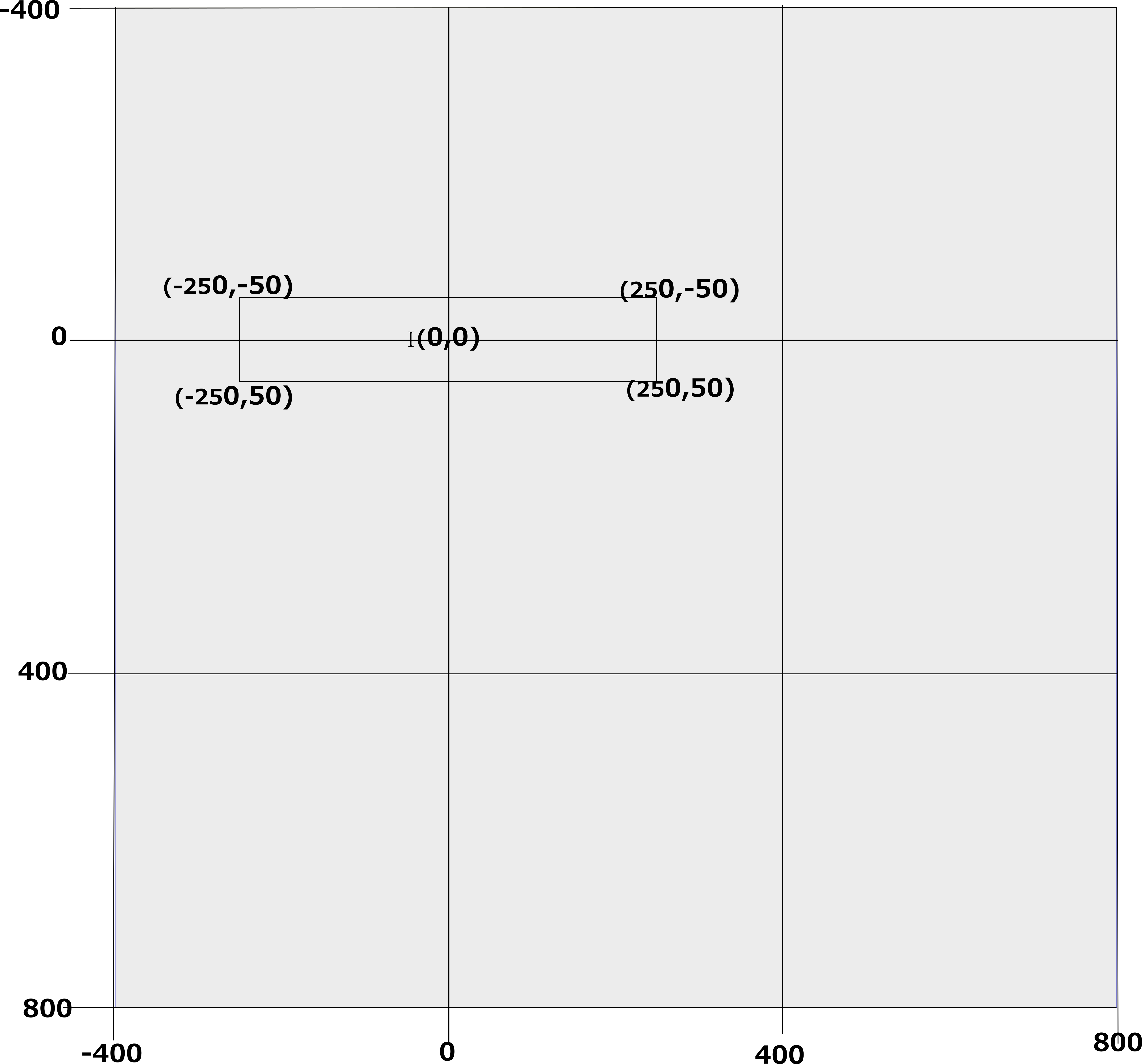
Here we see that we have now extended our working area out as far as (800, 800), which corresponds to the two dimensional list that we have been using. This area is highlighted in Fig 4 below.

To translate our shape its position above we simply add 400 to the x and y values of each of its coordinates

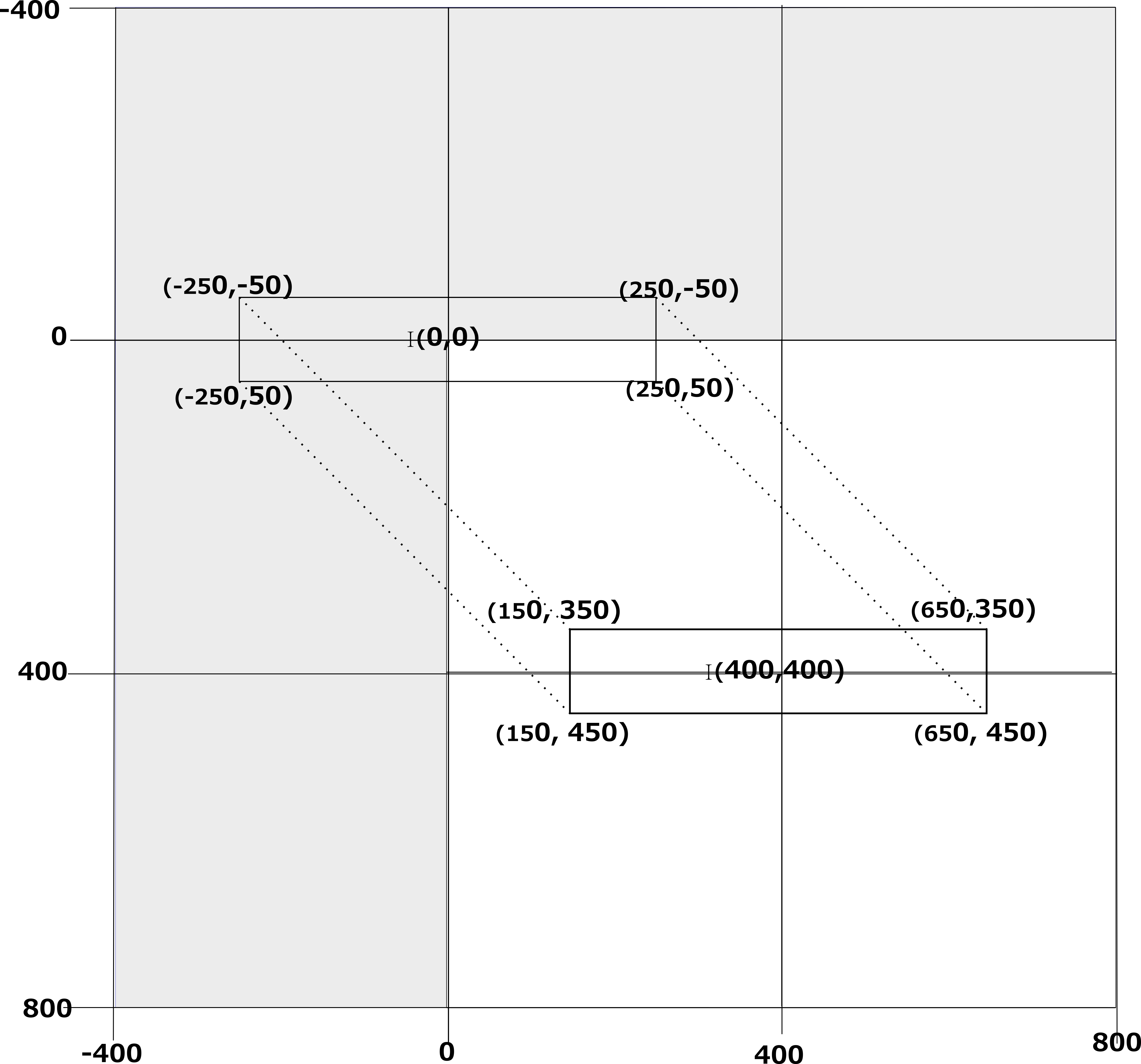
Here we see that adding 400 to the coordinates has moved our shape so that it is centered on the point (400, 400). Thus when the list is written to a PBM file our shape will be centerd.

Drawing a shape

The three code listings below are of the one function, drawShape(). The function has three distinct areas: setting up the base angle, calculating the four vertices of the shape and storing the values for the vertices in a two dimensional list.

As each section of the code is fairly intricate, it was decided to break it up into the different listings and explain each listing separately.

                        def drawShape(currentAngle,maxRows, maxCols):
                            a1 = 250
                            b1 = -50
                            hyp = math.sqrt(a1**2 + b1**2)
                            tangent=b1/a1
                            angle=math.atan(tangent)
                            angleD=math.degrees(angle)
                    

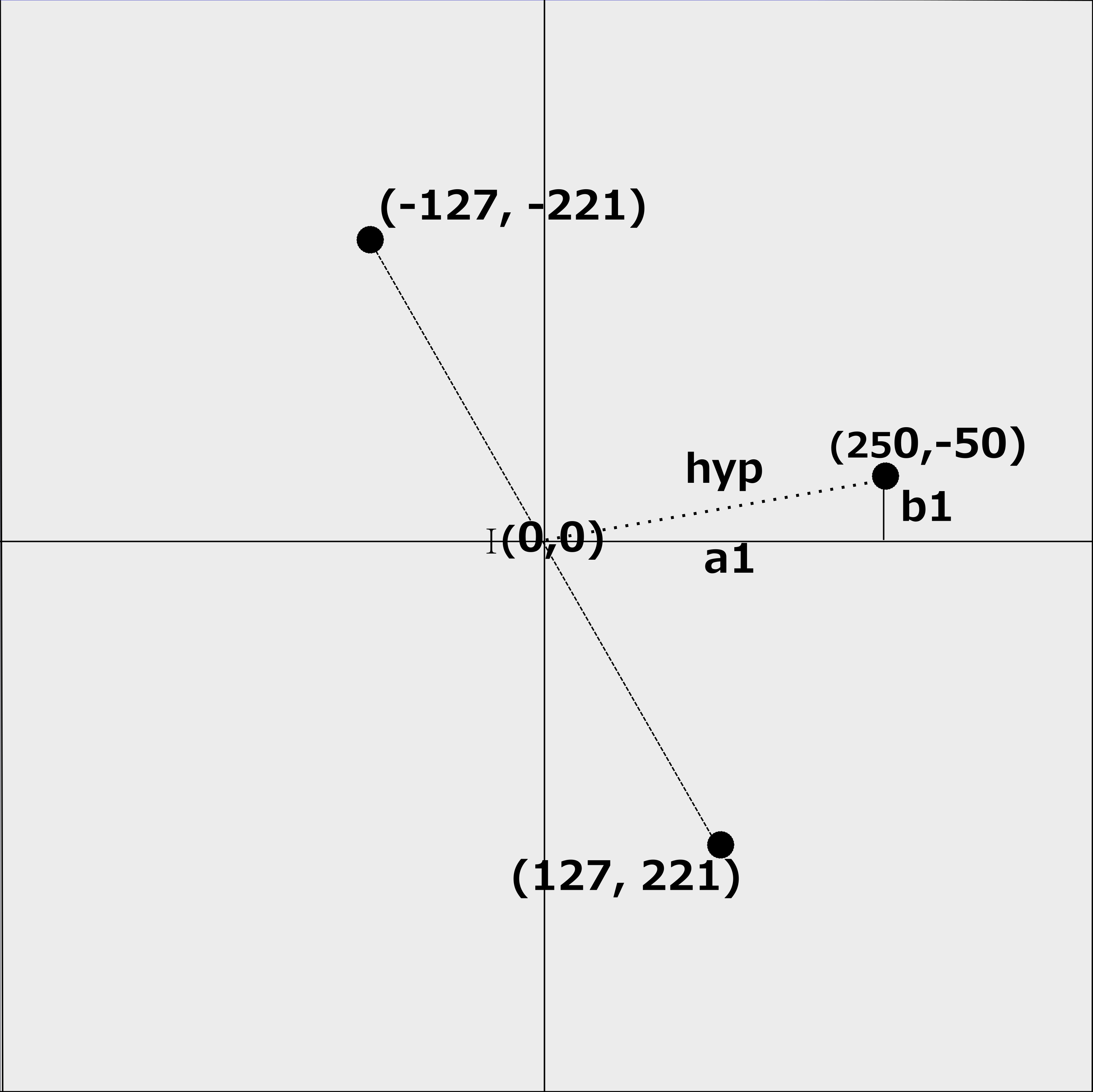
Before drawing our shape we need to determine the size of the angle between the diagonals of the quadrilateral.

At lines 13 and 14 we define two variables, a1 and b1 has having values 250 and -50 respectively. These are shown in Fig 6.

From these values we can calculate the hypoteneuse using Pythagoras' theorem. This works out at 255 when rounded

At line 16 we calculate the tangent of the angle by dividing the oppoiste by the adjacent. In this case it will be -50/250, which will be -0.2.

At line 17 we calculate the actual angle itself using Python's atan() function. This, however, returns the angle in radians. For this reason we need to use Python's degrees() function to convert the radian values into degrees. The value in this case will be -11.3 degrees.

We shall now examine the second part of our function, i.e. where we calculate the coordinates of the four vertices of our quadrilateral. In our application this function will be called 60 times. At each calling a new angle will be passed to it through the argument currentAngle at line 12 of Listing 1.1 above.

We cannot possibly run through the code 60 times, each time with a new angle. Instead we shall run through it once where the value passed to the argument currentAngle is 60 degrees.

                        
                            ang = currentAngle
                            rang = math.radians(ang)
                            x1 = math.cos(rang) * hyp 
                            y1 = math.sin(rang) * hyp 
                            x3 = -1*x1 
                            y3 = -1*y1 
                            nx1=round(x1)+400
                            ny1=round(y1)+400
                            nx3=round(x3)+400
                            ny3=round(y3)+400
                            
                            ang = currentAngle + angleD
                            rang = math.radians(ang)
                            x2 = math.cos(rang) * hyp
                            y2 = math.sin(rang) * hyp
                            x4 = -1*x2
                            y4 = -1*y2
                            nx2=round(x2)+400
                            ny2=round(y2)+400
                            nx4=round(x4)+400
                            ny4=round(y4)+400
                    

At line 20 the value of currentAngle is copied to ang. We presume this to be 60 degrees. At the next line this value is converted to radians and stored in the variable rang. This strange variable name is meant to be "Radian Angle".

With our angle converted to radians, we can now proceed with calculating the coordinates of our quadrilateral.

At line 22 the x coordinate of our first vertice is calculated as the cosine of 60 multiplied by the value of hyp. This is equivalent to multiplying 255 by 0.5 giving 127 when rounded.

Similarly at line 23 the value of the y coordinate is calculated as the sine of 60 multiplied by 255. Again this is equivalent to multiplying 0.8660 by 255, giving 221 when rounded. These will be stored in the variables x1 and y1.

Lines 24 and 25 calculate the values of x3 and y3 by multiplying the values of x1 and y1 by -1, thus giveing us vlaues of -127 and -221.

By now we have the coordinates of the first diagonal of our quadrilateral complete, as shown in Fig 7 below.

Calculating the coordinates of x2 and y2 is done in the exact same way as their predecessors. The only difference is that we shall be using a different angle. The new angle will be the sum of currentAngle and angleD, which will be 60 - 11.3 giving an angle of 48.7 degrees.

With this new angle value lines 32 to 36 calculate the values of x2, y2, x4 and y4. These values are 168, 192, -168 and -192.

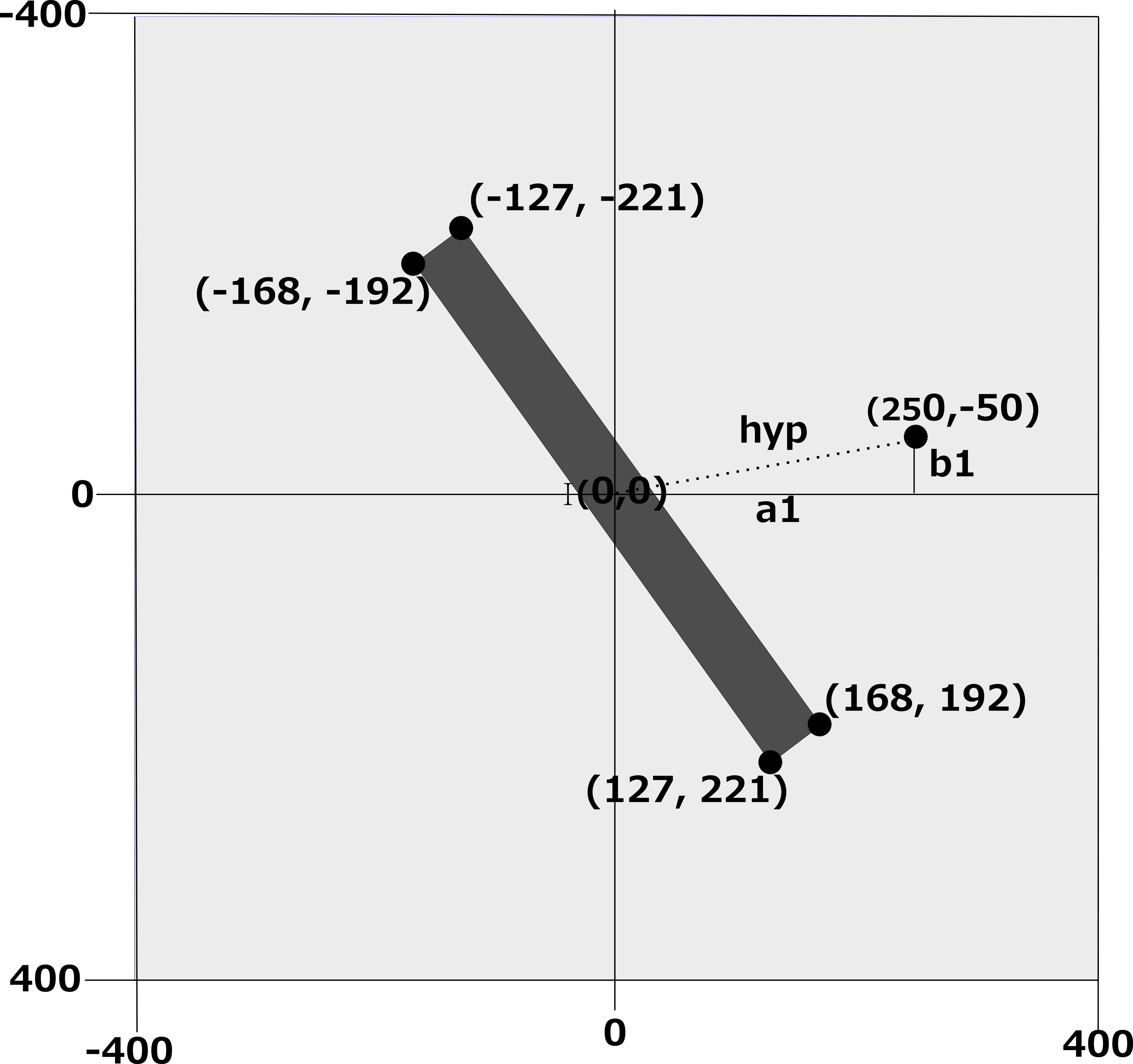
Fig 8 shows the complete set of coordinates for our quadrilateral and how the shape itself might look when saved to a PBM file.

Our job is not complete yet however. A half of them are negative, which means that they are not yet compatible with our two dimensional array. The other issue is that they are real number and not integers. We must therefore convert them to integers using the round() function and add a value of 400 to each one. This is done in lines 26 to 29 and 37 to 40 of Listing 1.2.

                            shape = []
                            coord = []
                            coord.append(round(nx1))
                            coord.append(round(ny1))
                            shape.append(coord)
                            coord = []
                            coord.append(round(nx2))
                            coord.append(round(ny2))
                            shape.append(coord)
                            coord = []
                            coord.append(round(nx3))
                            coord.append(round(ny3))
                            shape.append(coord)
                            coord = []
                            coord.append(round(nx4))
                            coord.append(round(ny4))
                            shape.append(coord)
                            
                            return shape
                    

We now have eight values for our coordinates that we must pass back to the calling function. The simple way to do it is to pass the data back as elements within a list. A two dimensional list is initialised and populated above at lines 42 to 58. The entire list is then returned at line 60

The main function

                        def main():
                            arrPage = []
                            strFileName="Rotate"
                            intVersionNumber = 0
                            intMaxCols=800
                            intMaxRows=800
                            for angle in range(0, 181,3):
                                arrPage = createBackground(intMaxCols,intMaxRows)
                                arrPage = fillShape(arrPage, drawShape(angle,400,400), intMaxRows, intMaxCols)
                                saveFile(arrPage,intMaxRows, intMaxCols,strFileName, intVersionNumber)
                                intVersionNumber+=1
                                arrPage=[]
                        
                        if __name__ == "__main__":
                            main()
                        
                        print("Programme finished")
                    

In this function we only need to look briefly at lines 114 and 116.

In the previous section we took a detailed run through the function drawShape() using 60 as the value of our angle. Line 114 is our for loop. It iterates in steps of three from zero to 180. It will therefore iterate 61 times. The value of the loop counter angle determines the tilt of the first diagonal of our quadrilateral. Therefore as the loop iterates for each frame the tilt of the first diagonal will have the values 0, 3, 6, ..., 174, 177, 180.

At lines 116 the function fillShape() is called. Its second argument is a call to drawShape(), the function we have been looking at. Also in the call to drawShape() the value of the loop counter angle is passed as an argument.

As you can see from line 60 of Listing 1.3 the function drawShape() returns a list containing the adjusted values for the vertices of our quadrilateral. The function fillShape() uses the data in the list as reference when filling in the area inside the quadrilateral.

End product

When we did a detailed runth through the function drawShape() we used the value of 60 degrees for our angle. Below we show below the single frame that would be created for that angle.

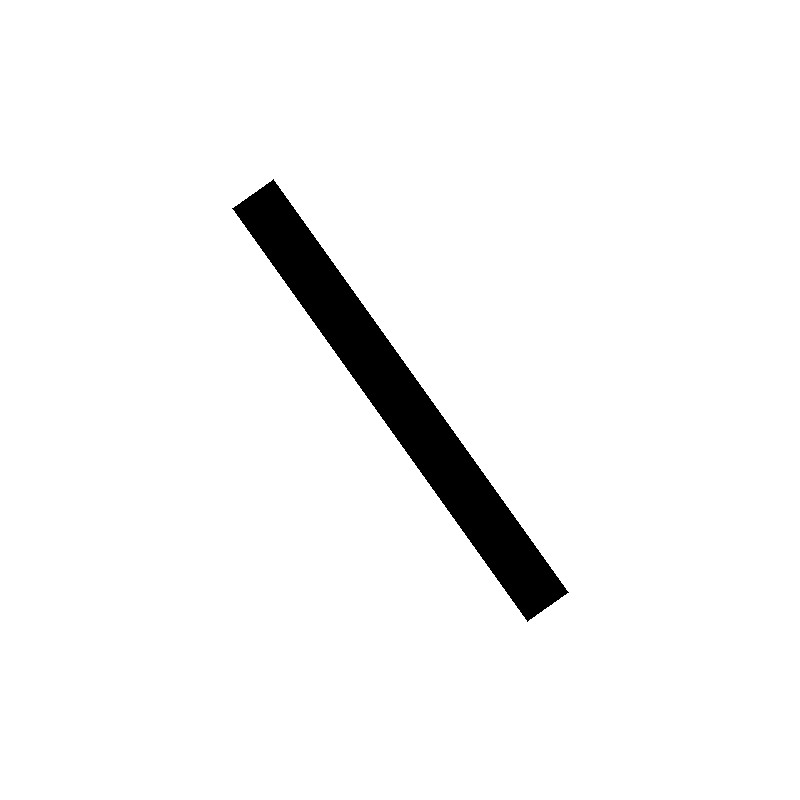
Notice the similarity between this image and Fig 8.

Going through it 61 times, with a different angle value each time, will give us 61 frames. Using those frames to create a GIF file will give us a more interesting result as can be seen in Fig 10 below.