Sudents are expected to have thorough knowledge of coordinate geometry including calculating the gradient of a line, secifying the line's equation and plotting the coordinates of points on the Cartesian plane.
The students must also be able to solve linear equations.
This block contains Python code that simulates movement and colour processing in cpmputer graphics and animations. It is meant to be supplementary material for the following NCEA modules:
91896 Use advanced programming techniques to develop a computer program
91906 Use complex programming techniques to develop a computer program
91908 Analyse an area of computer science
In the Level 2 and Level 3 programming modules the code could be used as examples of complex processing of lists.
In the Level 3 Computer Science module it could be used as a reference for the Computer Graphics option.
In the area of Computer Science, graphics is not related to image processing such as using Photoshop or GIMP. It relates to studying the concepts of how digital data is used to produce colours and shapes in images such as .jpg or .png files.
Since .jpg and .png files contain a fairly large amount of data, our examples use the very simple .pbm files when dealing with pure black and white and the more complex .ppm files when dealing with colour.
PBM files, like .jpg, or .png files, can be opened with image processing software such as GIMP or Adobe Phtotshop. Unlike both GIMP and Adobe Phtotshop, they can also be opened and processed with text editors such as Notepad or Notepad++.
Like any raster files they are composed of pixels. In the case of PBM files, however, the values of the pixels are limited to two values: 0 to represent white pixels and 1 to represent black pixels. By carefully arranging 1's and 0's in the file black shapes on a white background can be traced.
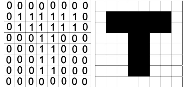
Fig 1: Two views of the PBM file
The left view shows the contents of a PBM file as it would appear in a text editor such as Notepad. The right view shows the same file as it would appear in an image processing software like Photoshop. Of course as the sample image is only 8 pixels wide and 8 pixels long, it would hardly be visible on the screen unless zoomed in on.
At the start of the file, before adding the 1's and 0's we need to provide three items of information to inform image processing software of the file's structure.
The first piece of information provided is 'P1' which informs the software that the file is a PBM file. The next two pieces of information are two integers indicating the number of columns and the number of rows in the file. The start of our sample file would look as follows:
P1 8 8
This would signal to the opening software that this was a PBM file with 8 columns and 8 rows.
In the PBM files on the following pages the file sizes are 800 pixels X 800 pixels and thus the two top rows would be:
P1 800 800
For more information on PBM files follow the link in the footer for the Lifewire TECH FOR HUMANS website
PPM files work on the same principle as the PBM files, apart from one big difference: the PPM files can process full colour. This means that they will be much larger than the PBM files
Instead of a single bit representing 1 or 0, the PPM files use three bytes to represnet the RGB colour system. Colours can be manipulated by changing the values of the red, green an blue components of the different pixels.
Since data for the three primary colours will be stored in a list, processing a PPM file will involve processing a three dimensional list.
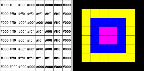
Fig 2: Two views of the PPM file
Instead of 1's and 0's we use the hexadecimal code for colours in the PPM files.
Comparing the two different views we see that in the image at the left #000, which is the code for black is in all of the pixels around the edge.
In the next layer has #ff0, the code for yellow, is in all of the pixels. This is followed by #00f, the code for blue and finally by #f0f, the code for magenta.
For the PBM files all of the programs use two dimensional arrays of 800 X 800. Each item in the array represents a pixel.
For drawing the shapes it was decided to use Cartesian geometry in order to draw on the students' prior knowledge of that topic. Introducing them to Bresenham's Line Algorithm would, it was felt, increase the cognitive load.
Before looking at the actual code for drawing shapes, let us first look at how the Cartesian plane is represented on the computer screen.
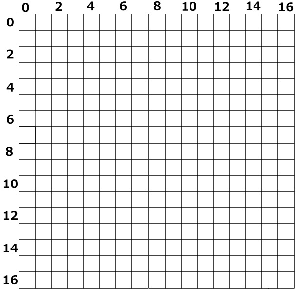
Fig 3: no shapes have been drawn
Above we have a view of an empty Cartesian plane that we shall be using in our exercises for drawing.
The most obvious difference between it and the version used for coordinate geometry in a Mathematics class is that the x axis is at the top. The other difference is that there are no negative values in either of the x or y axes.
The fact that we are restricted to positive values in the two axes does not hinder us in any way. We can always enter negative values for coordinates of points and the software can then adjust the entered values to positive ones, before drawing the shapes.
Before writing code for manipulating the 800 x 800 pixel PBM files we shall first look at writing simple programs than can produce coordinates for drawing vertical, horizontal and a variety of sloping lines.
The coordinates produced can then be used to colour in the points of a line, using a grid like that shown in Fig 3 above.
In the case of a horizontal line the values of y remains constant, regardless of the value of x.
We shall look at how to draw a line from (0, 8) to (0, 16).
First we work out the gradient of the line using the formula m = (y1-y2)/(x1-x2). In this case this works out as m = (8-8) / (16-8) = 0
The equation of a line is calculated as y1-y2 = m*(x1-x2). This works out as y1-8 = 0*(x1-16)
This is the same as y1-8 = 0
Taking the 8 over to the other side we get y1 = 8
We can test the equation above on value of x between 0 and 16. This is shown in Listing 1 below.
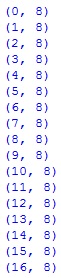
Listing 1: Code for a horizontal line
                            for x in range(0, 17):
                                y = 8
                                print(x, y)
Running this program will give an output as shown below.
Fig 4: the list of coordinates for points on our line
Once we plot the list of coordinates of Fig 4 above onto our grid, we get a result as shown below.
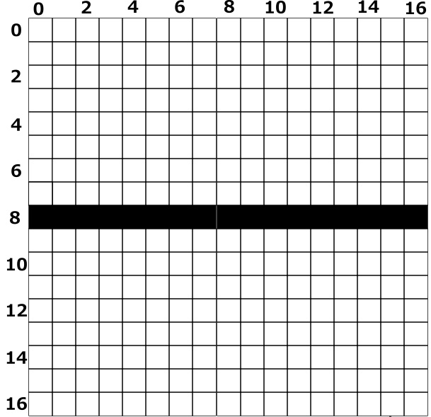
Fig 5: since y stays at a constant value of 8 the graph is a horizontal lineGo to top
Vertical Line
In the case of a vertical line the values of x remains constant, regardless of the value of y. For our example here we shall look at drawing a line between the points (8, 0) and (8, 16).
Trying to get the gradient of the line using the formula m = (y1-y2)/(x1-x2) we end up with (0-16)/(8-8).
Here we are trying to divide by zero which is not possible, and thus we shall have to try another formula
The standard formula for the equation of a ine is:
y1-y2 = m*(x1-x2)
Multiplying out we get y1-y2 = m*x1-m*x2
Swapping the values we get -m*x1 = -y1 + y2 - m*x2
Multiplying across by -1 we get m*x1 = y1-y2+m*x2
Dividing across by m we get x = (y1-y2)/m + x2
The gradient m has a value of (y1-y2)/(x1-x2). In the above expression we are dividing with it and therefore the expression can be rewritten as x = (y1-y2)*(x1-x2)/(y1-y2) + x2
Since both x1 and x2 have a value of 8 the expression x1-x2 has a value of zero. Consequently our last line can be rewritten as x = x2
Since x2 has a value of 8 then our formula ends up as x = 8
Since x in this case has a constant value of 8, we need to make y the subject of the formula, as shown in Listing 2 below.
Listing 2: Code for a vertical line
                            for y in range(0, 17):
                                x = 8
                                print(x, y)
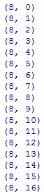
The output of this listing is shown in Fig 6 below. Notice that the x value in all of the coordinates is 8
Fig 6: Output from Listing 2
When the coordinates from Listing 2 are mapped on to our grid we get a display like Fig 7 below.
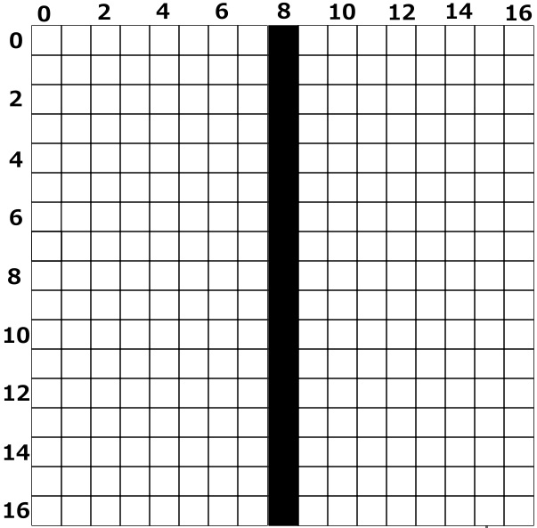
Fig 7: x has a constant value of 8 regardless of the value of yGo to top
Diagonal Line
For our example of a diagonal line we shall draw a line between (0, 16) and (16, 0). Our first step is to calculate the gradient of the line. This will work out as: m = (16-0)/(0-16) = 16/-16 = -1
With a gradient of -1 we can now work out the equation of the line, which will be y1-y2 = -1*(x1-x2)
Substituting the values we get y1-0 = -1*(x1-16)
This gives us the general equation for the line which is y = -1*(x-16).
The equation is used in the code below in Listing 3.
Listing 3: Code for a diagonal line
                            for x in range(0, 17):
                                y = -1 * (x - 16)
                                print(x, y)
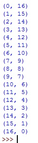
When run the code gives us a set of coordinates as shown in Fig 8.
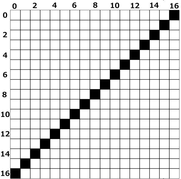
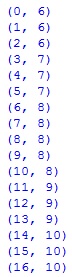
Fig 8: the output from Listing 3Fig 9: a diagonal line
The line is produced by plotting the coordinates from Fig 8 onto the grid.
What we refer to here as a gentle gradient are gradients that are greater than -1 and less than 1. Their main feature is that they can be fully graphed along the X axis. Here we are going to attempt to draw a line between (0, 6) and (16, 10)
We calculate the gradient as (6-10)/(0-16) = -4/-16 = 0.25
From this we can calculate the equation as follows y1-10 = 0.25*(x1-16)
This can be adjusted by taking the -10 across to y1 = 0.25*(x1-16)+10
This is what we have in line 2 of Listing 4 below.
Listing 4: equation of a gentle slope
                            for x in range(0, 17):
                                y = .25 * (x - 16)+10
                                print(x, y)
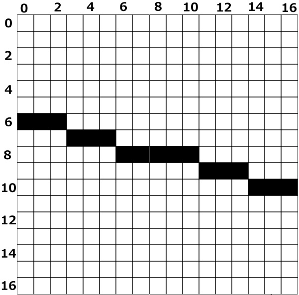
Fig 10Fig 11: a stepped line with a gradient of 0.25
Fig 10 above shows the output from Listing 4 The reason for the stepping in the line is that pixels cannot be broken down to sub parts, therefore the y values must be rounded to the nearest integer values. With a gradient of 0.25 the values of y are increasing much slower than that of the x, many of the y values will be the same while the x values change continuously.
In this example we wish to draw a line from (6, 16) to (14, 0). The gradeint will be calculated as (16-0)/(6-14) = 16/-8 = -2
The equation of the line is calculated as y1-0 = -2*(x1-14)
This tidies up as y = -2*(x-14)
As in the other examples this forms line 2 of Listing 5 below
Listing 5
                            for x in range(6, 15):
                                y =  -2*(x - 14)
                                print(x, y)
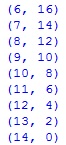
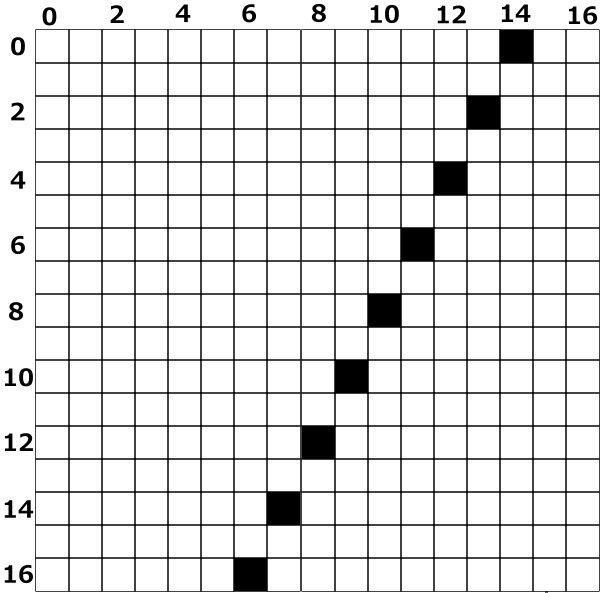
Fig 12
Fig 12 is the output of Listing 5. You can see that y is changing two units where x is changing by a single unit. For this reason there are gaps in the values for y. This can be seen in Fig 13 below.
Fig 13: the wider range of y is shown up as gaps in the lineGo to top
Steep Gradient: solid line
Here we look at plotting the same line as the previous example but being able to fill in all of the gaps. We will end up with a solid, albeit wonky line. As before we will be drawing the line from (6, 16) to (14, 0). We will however be reversing the roles of the x values and the y values.
As always our forst task is to get the gradient, but this time the formula will be (x1-x2) / (y1-y2) In this case that will be (6-14)/(16-0) = -8/16 = -1/2
Again to get the equation of the line we need to reverse the x and y coordinates. Thus the general formula for the equation is x1-x2 = m(y1-y2). In this case it will be x1-6 = -1(y1-16)/2
Taking the -6 across we get x1 = -1(y1-16)/2+6 = -1*y1/2+8+6 = ((-1*y1+28)/2)
Like its predecessors above this formula becomes line 2 of Listing 6 below.
Listing 6
                            for y in range(0, 17):
                                x =  ((-1 * y) + 28)/2
                                print(x, y)
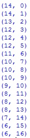
Fig 14
Fig 14 shows the output from Listing 6. If you compare it with Fig 12 you will notice that Fig 12 is a subset of Fig 14. Thus Listing 6 simply filled in the gaps left by Listing 5.
Fig 15: a wonky part of a straight line
Although the line in Fig 15 looks anything but straight, half of the points are actually on the line. The other pixels with black filling are approximate values that are used to make the line solid. What we have here is a strong close up of a larger image. If we were to draw this on and 800 X 800 grid, it would appear perfectly straight.
Here we introduced two image files that were pprobably new to you: .PBM and .PPM. The reason for their introduction is that they can be edited using text editors such as Notepad. As we shall see later they can be processed using Python code.
Apart from the files the rest of the page was about mathematics, especially coordinate geometry and linear equations. You should already be familiar with those topics so this was a quick revision on those two topics. Familiarity with those topics is necessary for successful completion of the rest of the following lessons
Download a copy or copies of the sample grid and use it to trace lines whose coordinates have been produced by Listing 4 as far as Listing 6. Tracing the lines means filling in with colour the pixels whose x and y coordinates correspond to those of the line.