Learning Outcomes
On completion of this lesson you will know to draw and animate circles.
Go to top
On completion of this lesson you will know to draw and animate circles.
Go to topHere we turn from quadrilaterals to circles. For the circles we need to use a different formula to what we used for quadrilaterals. We shall discuss the formula shortly.
Other than the formula we process circles in the same way as quadrilaterals. Firstly we build them up around the origin, (0, 0) for ease of processing and then we translate them to be centered on (400, 400).
We can animate them by moving them around the screen but rotating them around their own centre is a pointless exercise.
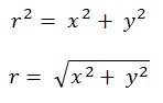
Above we have the standard formula for drawing the circumference of a circle or filling in the interior of a circle. Below we see it transformed into Python code.
r = math.sqrt(x**2 + y**2)
If this equation is true, i.e. if the square root of the sum of the square of x and the square of y is equal to r then the point (x, y) lies on the circumference of the circle.
r > math.sqrt(x**2 + y**2)
This states that if r is greater than the square root of the sum of the squares of x and y, then the point (x, y) is inside the circle. This is the version that we will be using in this lesson.
Go to top
                        for rad in range(200, 201,6):
                            arrPage = createBackground(intMaxCols,intMaxRows)
                            arrPage = drawCircle(arrPage, intMaxCols/2,intMaxRows/2, ra
                            saveFile(arrPage,intMaxRows, intMaxCols,strFileName, intVersionNumber)
                            intVersionNumber+=1
                            arrPage=[]
In this instance it is easier for us to look at a portion of the main() function in Listing 1.1 before looking at the function that fills in the circle.
The for loop at line 39 is set up to iterate only once with a radius value of 200 pixels.
The function drawCircle() is called at line 42. The values passed to it are the two dimensional array which is to be populated by the image of the circle, half of the value of the variables intMaxCols and intMaxRows and the radius of the circle. The reason for passing half the values of intMaxCols and intMaxRows is to specify the location for the centre of the circle. In this case it is meant to be (400, 400)
                        def drawCircle(arrPage, centreX, centreY, radius):
                            for x in range(radius * -1, radius + 1):
                                for y in range(radius * -1, radius + 1):
                                    if radius > round(math.sqrt(x**2+y**2)) :
                                        arrPage[round(x+centreX)][round(y+centreY)]=1
                            return arrPage
In Listing 1.2 at Line 12 is where we meet drawCircle(). Apart from the first argument which is our array, the values of centreX, centreY and radius are 400, 400 and 200 respectively. They are the values passed from line 41 of Listing 1.1.
Lines 13 and 14 form a nested loop where both iterate between the negavive and positive values of radius.
At line 15 we see the usage of the formula for determining if a point is inside a circle. If the value calculated here is less than the actual radius, this means that the point is inside the circle. If this is the case then control passes to line 16.
At line 15 calculations are made on the presumption that the centre of our circle is the origin (0, 0). However we want our circle to be actually centered on (400, 400). Hence at line 16 we add the values of the arguments centreX and centreY to the values of x and y. Thus if x and y had values of 40 and -50 respectively, the point that would be updated by line 16 would be (440, 350), which is well into the first quadrant. The value of 1 would be put into the appropriate element of the list corresponding to this point.
Once both loops have finished iterating, control returns to line 42 of the function main() where the data is saved to a file.
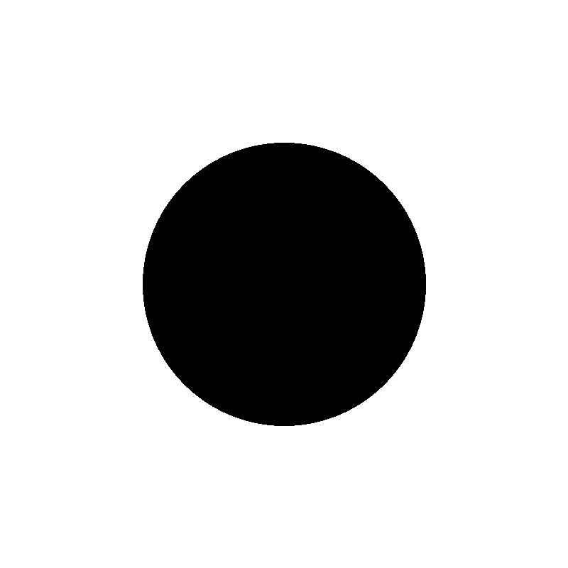
Fig 1 above shows our filled circle once the PBM file has been converted to a JPG file.
Download Program Code Go to topOur next example is simply a variation of the above. This time we are putting four circles on our page.
                        for rad in range(200, 201,6):
                            arrPage = createBackground(intMaxCols,intMaxRows)
                            arrPage = drawCircle(arrPage, round(intMaxCols/4),round(intMaxRows/4), 180)
                            arrPage = drawCircle(arrPage, round(intMaxCols/4),round(intMaxRows/4*3), 180)
                            arrPage = drawCircle(arrPage, round(intMaxCols/4*3),round(intMaxRows/4), 180)
                            arrPage = drawCircle(arrPage, round(intMaxCols/4*3),round(intMaxRows/4*3), 180)
                            saveFile(arrPage,intMaxRows, intMaxCols,strFileName, intVersionNumber)
                            intVersionNumber+=1
                            arrPage=[]
Lines 41 to 44 control each of the four circles. As well as the list arrPage the other three arguments are the x and y coordinates of the centre of each circle and the radius, which is 180. Thus the first circle is centered on (200, 200) and the other three on (200, 600), (600, 200) and (600, 600) respectively.
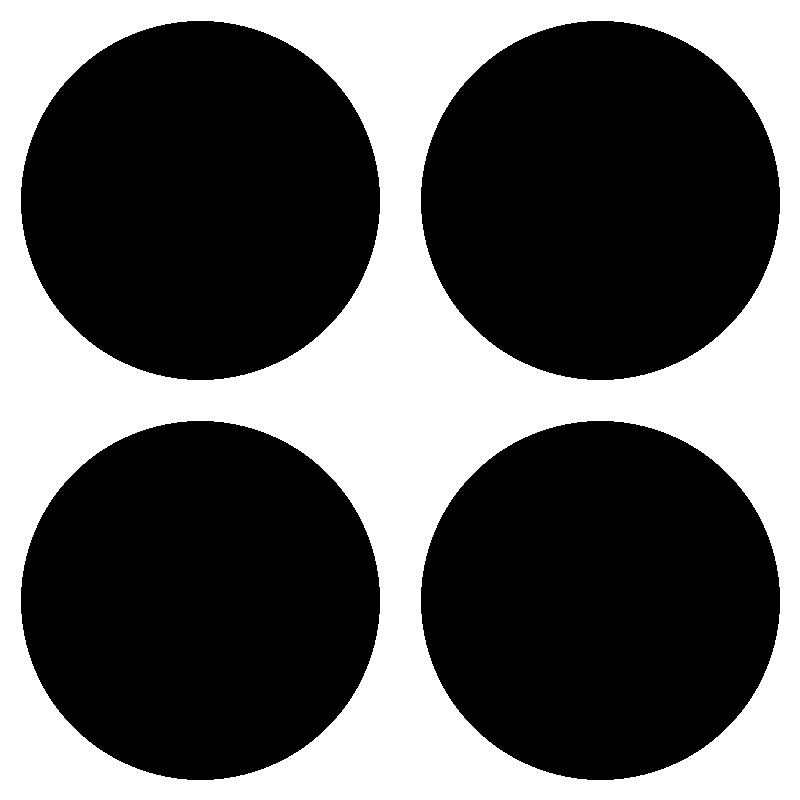
Fig 1 above shows the four circles.
This is simply avariation on the code from Listing 1.1 above, where the function drawCircle() is called four times instead of once. Also the radii of the four circles are reduced in length so that all four can be accommodated in the allowed space.
Go to topThis strange sounding term is the Latin word for 'ring'. In geometry it is the area between two concentric circles, i.e. circles with the same centre and different radii.
To draw it we need two circles with the same centre, then we plot the area between the two.
Our previous function drawCircle() will not work in this case as it would only fill both circles, which is not what we want. For this reason we have a new function, drawCircleBorder(), shown below in Listing 3.1
                        def drawCircleBorder(arrPage, centreX, centreY, longRadius, shortRadius):
                            for x in range(longRadius * -1, longRadius + 1):
                                for y in range(longRadius * -1, longRadius + 1):
                                    lengthOfLine = round(math.sqrt(x**2+y**2)):
                                    if longRadius >= lengthOfLine and  shortRadius <= lengthOfLine:
                                        arrPage[round(x+centreX)][round(y+centreY)]=1
                            return arrPage
Most of this function is identical to drawCircle() in Listing 1.1, apart from lines 12, 15 and 16.
At line 12 the function has one extra argument, which is the short radius, i.e. the radius of the inner circle.
At line 15 the distance between a point (x, y) and the origin (0, 0) is measured using the formula round(math.sqrt(x**2+y**2)). Here it is stored in the variable lengthOfLine.
At line 16 the variable lengthOfLine is tested for being less than the larger radius and greater than the smaller radius. If this is the case the point lies between the two circles and control passes to line 17.
Here, since we want our circle to be centered on on (400, 400), we add the values of centreX and centreY to the values of x and y in order to put the value 1 into the appropriate element of the list arrPage.
                        for counter in range(0, 1):
                            arrPage = createBackground(intMaxCols,intMaxRows)
                            arrPage = drawCircleBorder(arrPage, intMaxCols/2,intMaxRows/2, 300, 250)
                            saveFile(arrPage,intMaxRows, intMaxCols,strFileName, intVersionNumber)
                            intVersionNumber+=1
                            arrPage=[]
Here only lines 40 and 42 interest us. In line 40 the for loop is constrained to one iteration, since we only want a single image. At line 42 the values passed to drawCircleBorder() are the two dimensional list, the coordinates of the centre of the two circles, i.e. 400 and 400 in this case, and the value for the two radii, which are 300 and 250.
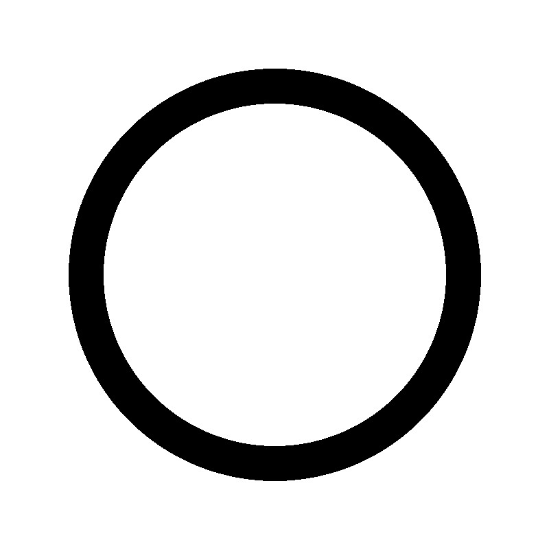
The image produced by the above code is shown in Fig 3.
Download Program Code Go to topFinally we look at animation of circles. With quadrilaterals we made them rotate around their own centre point as well as making them move around the screen. Rotating a circle around its own centre would be a pointless exercise, but we can make it move around the screen. In fact we can make a few of them run around in circles.
For our animation of the circles we don't need any more functions. Our old friend drawCircle() will do. There is however more processing than usual in the function main()
Our aim here is to have two circles oribiting around the central point of (400, 400). As each circle will be at oppoiste side of the centre to each other, the coordinates of their centres will be negatives of each other. We therefore need to calculate only one pair coordinates
                        def main():
                            arrPage = []
                            strFileName="RotatingCircle"
                            intVersionNumber = 0
                            intMaxCols=800
                            intMaxRows=800
                            for counter in range(0, 180,3):
                                arrPage = createBackground(intMaxCols,intMaxRows)
                                angle = counter
                                angleR = math.radians(angle)
                                xCoord = round(math.cos(angleR) * 240)
                                yCoord = round(math.sin(angleR) * 240)
                                xCoord1 = xCoord * -1
                                yCoord1 = yCoord * -1
                                arrPage = drawCircle(arrPage, xCoord,yCoord, 30)
                                arrPage = drawCircle(arrPage, xCoord1,yCoord1, 30)
                                saveFile(arrPage,intMaxRows, intMaxCols,strFileName, intVersionNumber)
                                intVersionNumber+=1
                                arrPage=[]

                        if __name__ == "__main__":
                            main()

                        print("Programme finished")
As line 41 inidcates, the loop counter controls the angle of the line from (400, 400) to the centre point of the circle. We can work out from line 39 the angles to the centre of the circle will be 0, 3, 9, 12, ... 168, 171, 174 and 177.
The distance between (400, 400) and the centre of the circle will always be 240, as indicated by lines 43 and 44.
At lines 43 and 44 the x and y coordinates of the centre of the first circle are calculated using the trigonometrical methods we have been using up to now. Lines 45 and 46 calculate the coordinates of the centre of the second circle by using the negatives of the first coordinates.
Since we have to draw two separate circles the function drawCircle() is called twice, first at line 47 and then at line 48. At line 47 the function is called with the values of xCoord and yCoord in the second and thrid arguments. These are the coordinates of the centre of the first circle. At line 48 it is called again, this time with the values of xCoord1 and yCoord1 in the second and third arguments.
Once the second calling of the function drawCircle() is finished all of the data for displaying two circles on opposite sides of the centre point of our image is complete. We only need to save it now. As always the saving is carried out by the function saveFile(), which is called from line 49.
Lines 50 and 51 tidy things up in readiness for the next iteration of the loop
On the next iteration the value of the angle will be three degrees greater than before and therefore the coordinates of the centres of the circles will be in slightly different positions to those in the previous frame.
This process continues until 60 frames have been created. The resulting GIF file is shown below.
In this lesson, we explored various techniques for drawing and animating circles. We started with the basic formula for determining if a point is inside a circle and then moved on to more complex shapes like annuli. We also discussed how to animate circles by making them move around the screen and how to create multiple circles in different configurations.
We provided several exercises to practice these techniques, including creating circle pairs at different angles and adding annuli to frames. These exercises help reinforce the concepts and provide hands-on experience with circle geometry and animation.
For further reading and more detailed information on circles, you can refer to the resources provided in the footer section.
Go to topThe block Multiple Circles is an extension of Filling a Circle. The code from the latter comes from the the downloadabe file 'Simple Circles.py'
Download that file and edit it as follows: replace line 41 with lines 41 to 44 of Listing 2 above. Once you run it, it should give an output like Fig 2 above
Modify Exercise 1 so that it shows 16 circles instead of four. To accommodate the larger number of circles the radii of all the circles must must be reduced so that they don't overlap.
Modify the function main() in Listing 4 above so that you will have two pairs of circles orbiting the centre instead of the current one pair. The steps for doing this are:
The extra code should be inserted between the current lines 48 and 49.
The result should look something like the example below.
Modify Exercise 3 so that you will have circle pairs at each 30 degree angle. This means circle pairs at 30 degrees, 60 degrees, 90 degrees, 120 degrees, 150 degrees and 180 degrees.
Add an annulus to your frame so that the circles appear to be running along the outer or inner edge of the annalus.
Extend Excercise 5 by adding an extra annulus to it. This should be positioned so that the circles are orbiting between the two annuli.
Go to top