Module: as91892 - Use advanced techniques to develop a database
Requirements: designing the structure of the data, using appropriate tools and advanced techniques to organise, query and present data for a purpose and end users, applying appropriate data integrity and testing procedures
Relevant Implications: end-user considerations
Advanced techniques: linking data in related tables or nodes using queries or keys, writing custom queries to filter and/or sort data, using logical, mathematical and/or wildcard operators, customising presentation of the data, using custom forms to add user input to the database, setting validation rules for data entry
In a real life application a table may have hundred or even thousands of records. Even a table like the school example we are using here may have up to a thousand records. A university version of the same table would have many thousands of records.
We rarely ever need to examine the contents of an entire table – we normally wish to look at only one record or else a small group of related records. Some examples of small groups of related records in our case would be:
The students in grade 12
The students in grade 11 who have paid less than K800 in fees
The New Ireland students who have paid the full fees
We nearly always work with small groupings like this and in order to allow us to separate the data we want from all of the data in the table we use queries.
As stated earlier we rarely want to look at all of the data in a table. We want to be able to reduce the number of fields we look at as well as the number of records. For our first example we shall look at all of the records but at only the fields surname, Name and Grade
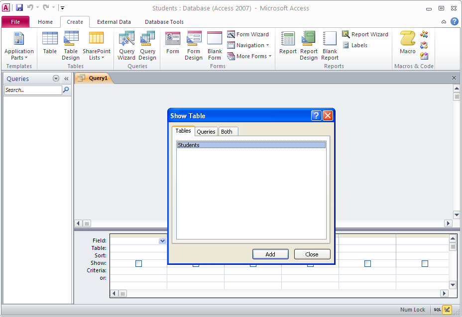
Fig‑1 below shows us the first step in designing a query for this. We click on the Create tab and then on Query Design in the Queries group. This brings up both the Query Design view as well as a dialogue box Show Table as shown in Fig‑1.
Fig 1
This dialogue box allows us to select the table whose data we wish to query. In our case our database contains only one table – Students – so we select that table and click on Add. Once we close the dialogue box our query design view will look as in Fig‑2
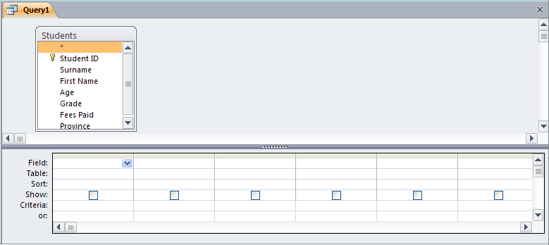
Fig 2
First we notice that the query design view is divided into two parts: the top part contains a box with the table name and the names of the fields inside the box, while the bottom half contains a grid that we shall use to build up the query.
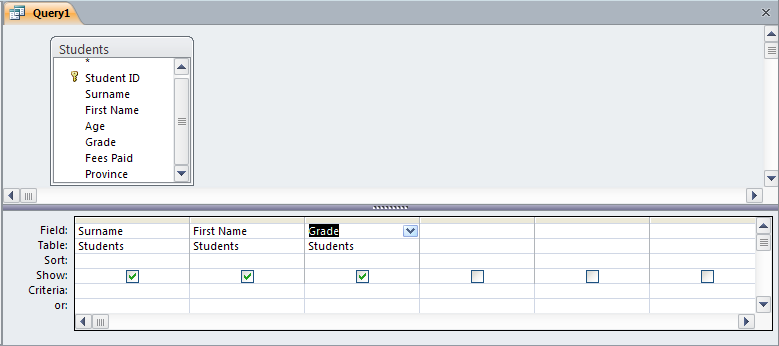
For our query we shall want only the values for the fields Surname, Name and Grade. In order to add those three fields to our query we either double click on each field name in succession or else we drag each field name down to the top row of the grid. Either way our query design will now look as in Fig‑3
Fig 3
Here we see that the first row, which is labeled Field, contains the names of the fields while the row below it simply contains the name of the table which contains the fields. The row labeled Show has tick marks underneath each field, indicating that they will be visible when we run the query. If we don’t want the field to be shown we simply uncheck this box.
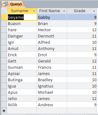
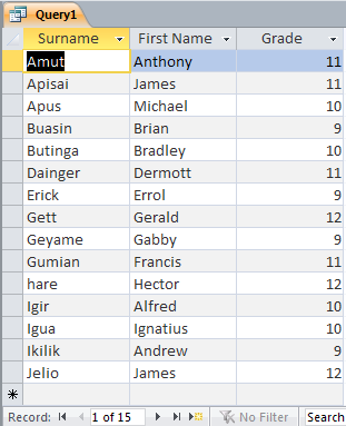
Running this simple query will give us a result as shown in Fig‑4.
Fig 4
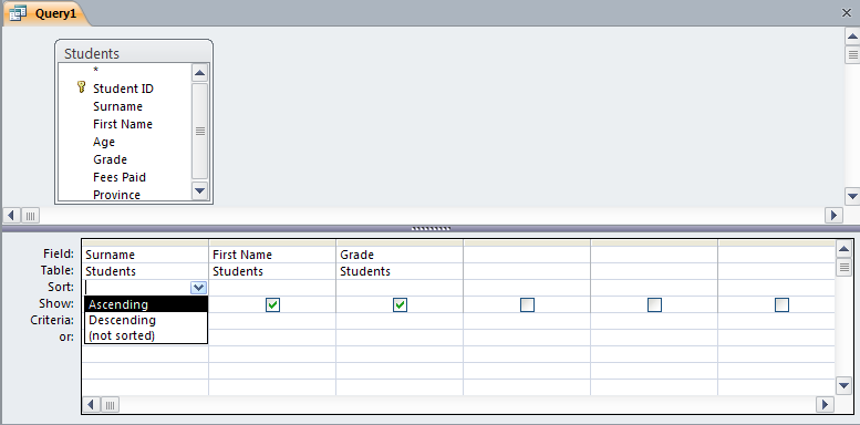
At first glance the data here seem to be in random order. This is because the table is sorted on the field Student ID, which is not included in the query and thus the records are displayed in the order in which they exist in the table. On the other hand if we wished to have the data sorted by surname then in the column allocated to Surname we would click in the Sort row as shown in Fig‑5 below. If we select Ascending and then run the query once more we get a result as in Fig‑6.
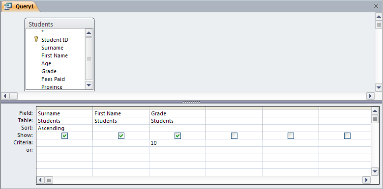
In the two versions of a query that we have done so far we have managed to limit the number of fields displayed but those three fields were displayed for all of the records in the table. But what if we only wanted the details of the students in Grade 10? In other words what if we only wanted to display the records where the Grade field contained the value of 10?
Fig 7
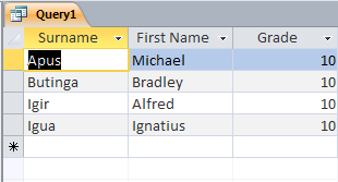
To do this we go back to the query Design view and in the row Criteria: we put in the value 10 in the Grade column as shown in Fig‑7. This tells the system to display only records with 10 in the Grade field. Now when we run the query again we get the result shown in Fig‑8.
The query that we have modified works fine for displaying the students in Grade 10. But what about the other three grades? One solution is to create three more queries – one for each grade. This would be acceptable in this case as we are dealing with only four grades, but what about if we wanted to use Province as a criteria? In that case we would need to create 19 different queries! And then once Hela and Jiwaka became provinces we would need to add two more. Clearly this is not an acceptable solution.
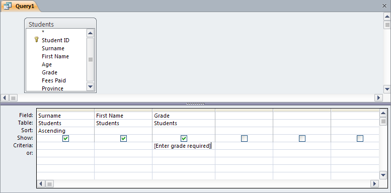
The best approach regarding our problem with the grades is to allow the user to interactively specify which grade they want displayed. In order to do that we modify the query again as shown in Fig‑9.
Fig 9
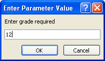
Here, in the Criteria: row under Grade we have simply entered a prompt enclosed in square brackets – [Enter grade required]. The result of this is that when we now run the query the first thing that happens is that a dialogue box appears as inFig‑10. Notice that the prompt in the dialogue box is exactly the same as the prompt we entered into the Grade column. If we enter 12 into the text box and press OK, then, when the query is run, it will be equivalent to having the value 12 in the Criteria row of the column Grade.
Fig 10
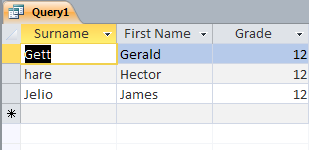
The results of the query is shown in Fig‑11. The next time we run the query if we were to enter 11 then we would get only the students where the grade field has a value of 11, or in other words we would get the students in Grade 11.
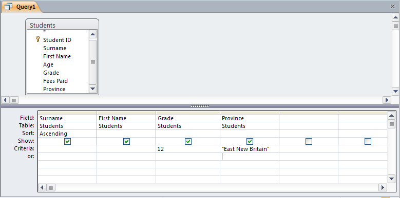
If we wanted a list of all of the grade 12 students who come from East New Britain, we would make a request to the system as follows: Select all of the records where the value of Grade is 12 AND the value of Province is “East New Britain”. In order to do this we have to make the following modifications to our query design:
we put the field Province into the query
in the Criteria: row we put in the value “East New Britain”
in the same row under Grade we put in the value 12.
Our design will now look as in Fig‑12.
Fig 12
When we run the query now, we get the result shown in Fig‑13. Notice that this is a subset of the result we got in Fig‑11. The number of records are smaller since the non East New Britain students have been filtered out.
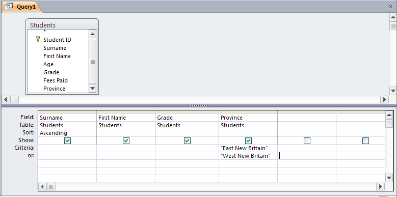
We use OR queries when we want to test the same field for different values. For example we may want to list all of the students from the both East and West New Britain provinces. In this case we are telling the system to select all of the records where the value of the Province field is either “East New Britain” or “West New Britain”. In order to do this we have to enter the names of those two provinces in the Province column at the Criteria: rows. This is shown in Fig‑14.
Fig 14
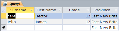
Here one province name is entered in the Criteria: row itself and the second name is entered in the or: row underneath it. As you may be able to work out from this diagram we can enter as many province names as we wish in the rows underneath, or in other words we can have as many or’s as we need. When we run the query this time with the two province names as criteria, we get the result in Fig‑15.
In our table we have a field for fees paid. This shows only the amount that have been paid so far. We also may wish to find out how much people owe in fees. This can be easily calculated by subtracting the current value of the field from the total fees. This could be added to the table but this would involve extra data entry as well as extra storage space. It is much more efficient to allow a query automatically calculate this for us.
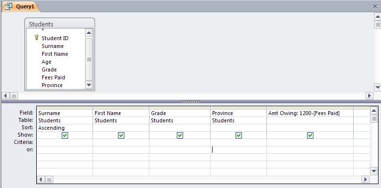
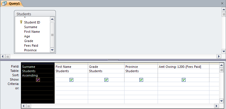
For our example we shall presume that the total fees is K1,200. The amount owing should, therefore, be 1200 less the value of the field Fees Paid.
Fig 16
Fig‑16 above shows us how this is achieved in the query design. The first step is to enter the name of the field – Amt Owing in this case. This is followed by a colon and then by the actual calculation, 1200 – [Fees Paid]. What this means is for each record to subtract the value of the field Fees Paid from 1200 and to store the result in the new field, Amt Owing.
We notice above that the name of the field Fees Paid is enclosed in square brackets. The reason for this is that it has a space character in it. When this is the case then, when we are entering a formula, we include the entire field name in square brackets to indicate to the system that it is a single unit. If the name of the field is a single word i.e. Name, Surname or Grade then we don’t need to put those into square brackets but when we have completed entering the formula the system itself will put square brackets around the field names.
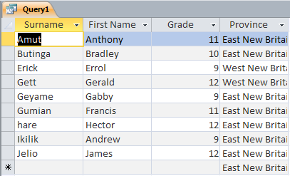
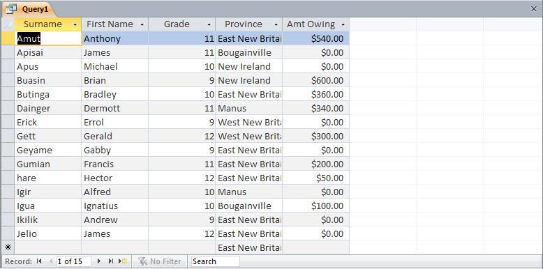
In this case we have also added a criterion to this field so that only records with values greater than zero are displayed. The result of running this query is shown in Fig‑17.
Fig 17
Later in the chapter Reports we shall be using this query as a basis for a sample report.
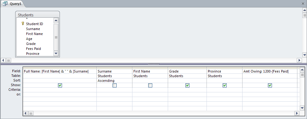
For our example here we shall add the contents of the two fields Surname and Name together in one field so that the student’s name will look a bit more natural. As we would like this field to appear at the leftmost column we must insert a blank column to the left of the column Surname.
Fig 18
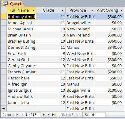
To insert this new column we must first select the existing column Surname as shown above and in the Design tab click on Insert Column. This will create a blank column for us to enter our new calculated field. The name of this field will be Full Name and the calculation will be [Name] & “ “ & [Surname]. Let us spend some time examining this text manipulation. Firstly the ampersand symbol - & - ties two pieces of text together. Thus “John” & “Smith” would give us “JohnSmith”. Of course this is not what we want – we need a space between the two words and thus the correct version would be “John” & “ “ & “Smith”, which will give us “John Smith”. The full formula is shown in Fig‑19. We do not need to print the contents of the fields Surname and Name and thus we uncheck the tick boxes below them in the row Show:. The result of running this query is shown in Fig‑20
Most of the time queries are temporary entities, or, in other words, the data exists in them only as long as the query is running. Once a query is closed down the data in it disappears. Data is permanent only in tables.
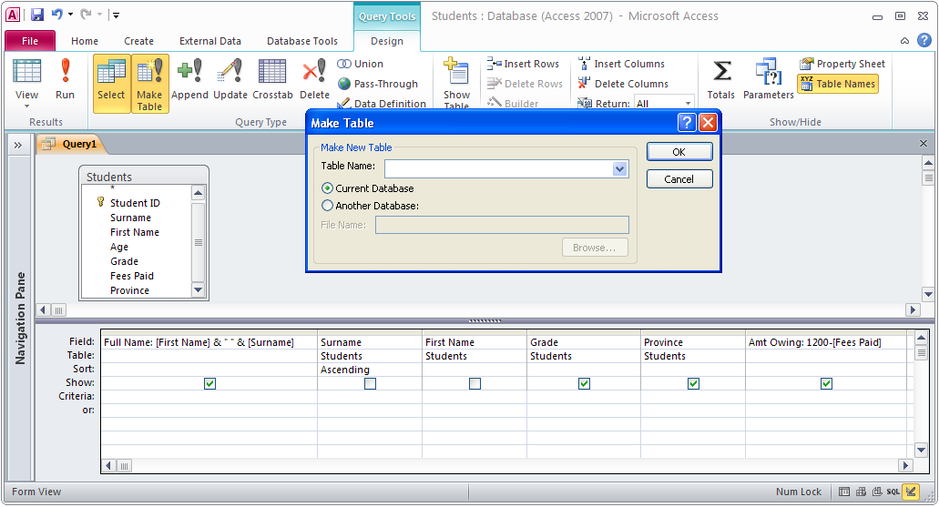
If we wish to make a query’s result permanent we change it into a Make Table query. For our example we shall use the query above, which prints out students who still owe money.
The first step is to open the query in Design mode. In the Design tab click on the icon Make Table. This brings up the dialogue box shown below. Here we specify whether we want to export the new table to another database or whether we want to save the table in the current database. In our case we select the current database. Next we enter the name the table, which will be Students who own money and click on OK.
Fig 21
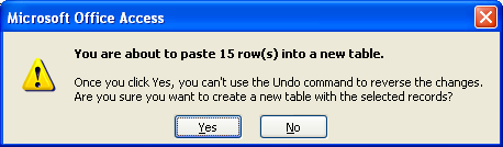
Next we have to run the query. When we do no results are displayed on the screen. Instead we get the dialogue box shown in Fig‑22, asking us to confirm that we wish to add record to a new table. Once we click on Yes the new table is created and the results of the query are stored in it.
Fig 22
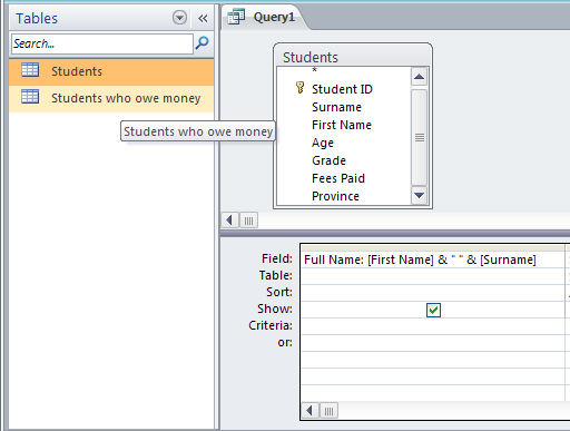
If we now look at the database window we see that a new table has been added as shown in Fig‑23.
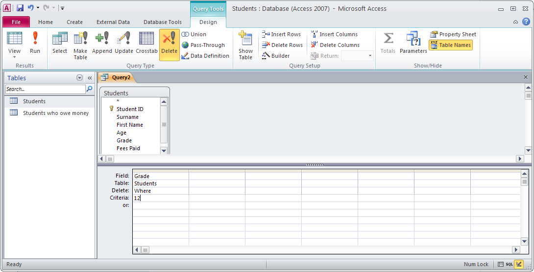
At the end of the school year we need to get rid of the records of our grade 12 students as they are leaving the school. Rather than manually going through the database and deleting each grade 12 record we can create a delete query that will do the job for us more quickly.
To do this we first create a normal query but put only one field into it – Grade – as shown in Fig‑24. Next we click on the icon Delete in the Design tab. This removes to Sort row from the quey design window and replaces it with Delete. Now the logic of the query can be read as delete from the table Students all records where the value of Grade is 12.
Fig 24
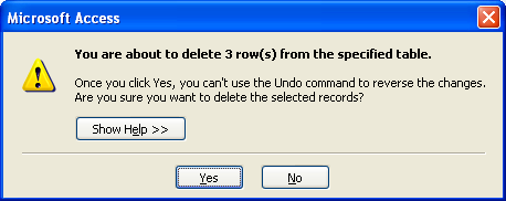
When we run the query we get the dialogue box shown below. If we click Yes then all of the records where the value of the Grade field is 12 will be deleted.
Fig 25
If you run the query a second time the message will start You are about to delete 0 row(s)… since all records with 12 in the grade has already been deleted and there are no more left to delete. If you check your table by opening it you will see that all records for grade 12 are gone.
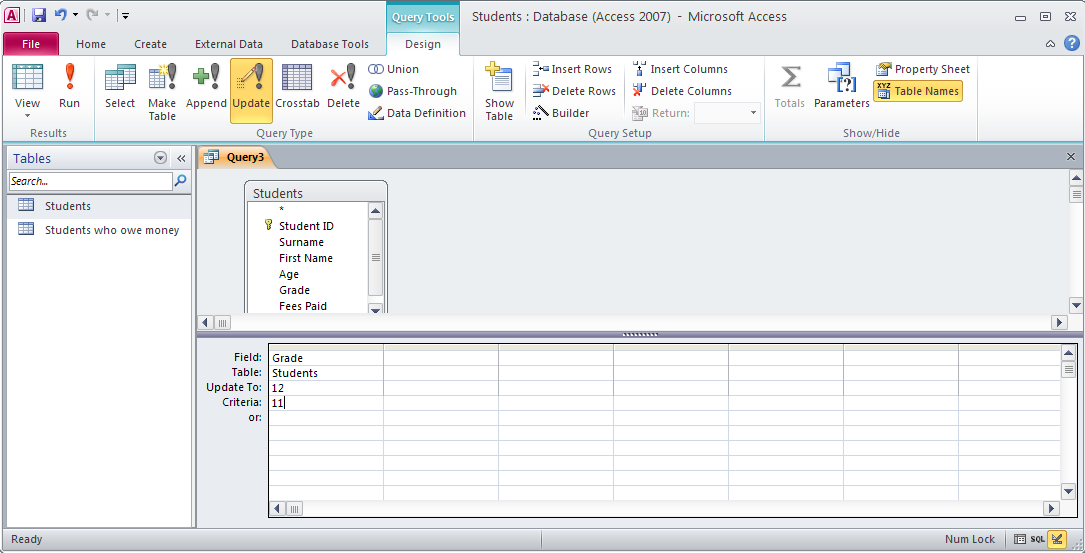
An Update query is one that changes the values in the fields of one or more records in a table. As an example of this query we shall follow on from the delete query example above. There we deleted all of the grade 12’s since they would be leaving the school. Consequently the current Grade 11’s would be updating to grade 12. Again, rather than manually changing all 11’s to 12’s we shall create an update query to do the job for us.
Fig 26
The design of the query is shown in Fig‑26 above. To begin it we again create an ordinary query and insert only the Grade field into it. Next we click on Update in the Design tab, which alters the display to that shown above. In the row Update to we insert the new value we want in the field. Next we enter 11 into the Criteria row to indicate that only the records with 11 in the grade field are to be updated to 12. If we left the criteria out then all records in the table would be updated to 12. The logic of the above query is equivalent to in the Students table update the Grade field to 12 where the original value is 11.
We could either create separate queries or modify our current one to update all of our grade 10’s to 11 and our 9’s’ to 10’s
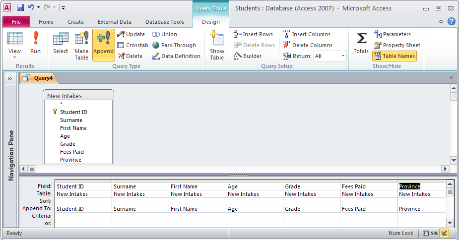
Append queries select data from one table and append it to another table. For our example we shall continue with the end of year processing we have been doing on our student table so far. We have already got rid of the grade 12’s and changed the current 11’s to 12, 10’s to 11’s etc. What is left for us now is to enter new grade 9’s.
Supposing that we have a list of our new grade 9’s in a table called New Intakes, then we want all of the data in this table to be appended to our Students table. We assume that this new table has exactly the same structure as the Students table. We shall look at creating an append query to do this.
This query is not run on the Students table, it is run instead on the New Intakes table. We start off the query as one that would print out all of the fields of all of the records in the table New Intakes. Next we go to the Design tab and click on the icon Append. This will alter the display to that shown in Fig‑27 below.
Fig 27
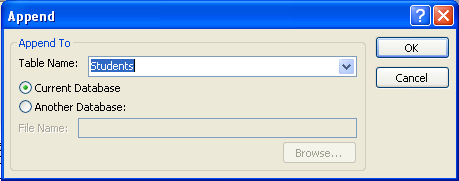
Next we run the query. This brings up the dialogue box below. For Table Name: we select Students and click on Current Database. Once we click on OK the data in the table New Intakes will be appended to the table Students.
Queries are a way for us to isolate the small amount of data we want from the enormous amount of data that can be stored in a database. Firstly we may not need all the fields of a table and thus we can specify which fields we want displayed by using the Criteria rows. As well as the fields actually in the table we can add extra fields to a query to display calculations based on data already stored in the table.
What is the primary purpose of using queries in a database?
To store all data in a table
To sort data in alphabetical order
To isolate and retrieve specific data
To create backup copies of data
Which design tool is used to visually create queries in a database?
Query Wizard
Report Builder
Design View
Table View
What does the "Criteria" row in a query design grid specify?
The fields to include in the query
The records to filter
The table names
The display order of records
What type of query is used to permanently save query results as a table?
Update Query
Delete Query
Make Table Query
Append Query
Which operator is used in a query to combine multiple conditions that must all be true?
OR
AND
LIKE
IN
In the formula `[Name] & " " & [Surname]`, what does the ampersand (`&`) symbol represent?
Mathematical addition
Combining text
Logical comparison
Column selection
What happens when you use the "Delete Query" function on a table?
It removes selected rows from the table
It clears all table contents
It renames the table
It hides rows without deleting them
How can you sort query results in ascending order based on a specific field?
Use the "Order By" option in the Criteria row
Select "Ascending" in the Sort row
Enable the "Display" checkbox
Use the "Group By" function
What is a practical use of calculated fields in queries?
To add new columns to the database table
To perform operations like summation or concatenation
To delete unnecessary data
To filter records based on conditions
What does an "Append Query" do in a database?
Adds new records to an existing table
Updates existing records
Removes duplicate entries
Deletes unwanted records
Fill in the blanks
In a database, a __________ is used to isolate specific data from a larger dataset.
The __________ row in the query design grid is used to filter records based on specified conditions.
A __________ query creates a new table to store the results of a query permanently.
The __________ operator is used in a query to specify multiple conditions that must all be true.
The __________ operator is used to test a field for multiple possible values in a query.
A __________ query removes rows from a table based on specified criteria.
The __________ function in queries allows for combining values from two or more fields into a single field.
The query design view is divided into two parts: the top part shows the table and field names, while the bottom part contains the __________ grid for building the query.
Using the __________ query, you can add data from one table to another table in a database.
In a calculated field, square brackets are used around field names when the field name contains __________ characters.