The manipulation of variables is at the heart of computer programming. To the non-programmer variables are associated with algebra. A typical algebraic problem would be as follows:
If x = 5 and y = 9, what is the value of 2x+3y?
The solution to this of course is that if x is 5 then 2x is 10, if y is 9 then 3y is 27. Thus the expression 2x+3y equates to 10+27 which is 37.
Programming variables are both similar to and different from their algebraic cousins.
The similarities are that programming variables can be manipulated in exactly the same way as we have manipulated the algebraic ones above. Another similarity is that at any one time both types of variables can only have one value, and once we change the value in a variable the previous value is lost.
As an example, if we changed the example above as follows: x = 6 and y = 12 then 2x+3y would be 12 + 36 = 48.
One of the differences is that algebraic variables use only one letter for its name whereas programming variables use whole words or word combinations.
Another difference between the two types of variables is that program variables are physically stored in the computers memory. Thus when we create a variable, first a block of memory is reserved for that variable, and that block is given a name. To show this we shall convert the example above into python code
Listing 1
First = 6Second = 12Result = 2 * First + 3 * Second print(“The result of the calculation is “,Result)
The code above is in standard Python but it is close enough to EdPy that it should be easy to follow, so let us analyse it line by line:
In the first line a block of memory is reserved. That block is referred to as First and the value 6 is stored there.
The second line is similar: a block of memory is reserved, named Second and the value 12 is stored there.
The third line is different. As before a block of memory is reserved and named Result. However instead of storing a value there as we did before, we now have an expression which we must first calculate. The calculation follows the normal rules of mathematics:
Multiply 2 by the value retrieved from the memory location named First
Multiply 3 by the value retrieved from the memory location named Second
Add the result of the two multiplications and store the result in the memory location named Result.
The video below provides a notional machine that further explains the workings of this piece of code.
For our first example of the use of variables we shall go back to our very first example where the robot described the perimeter of a square. In that example the robot moved forward the same distance every time. In the version we are going to develop here the distance traveled by the robot after each turn is going to be greater than the previous one. This means that we get a right angled spiral as shown in the illustration in Figure 1 below.
Figure 1
This is the algorithm which allows the robot to trace out this shape.
We have already met the code in Listing 2 earlier. It is a copy of Listing 2 on the page Sequence. It simply moves the robot around the perimeter of a square. It is included here so we can see that our next example in Listing 3 is simply a derivation of it, i.e. extra features hare added.
Line pairs 2, 3; 5, 6; 8, 9; 11, 12; in Listing 3 are almost identical to Lines 1 to 8 from Listing 2; they simply move the robot and turn it. The only difference is that the last argument given to the Ed.Drive() commands at lines 2, 5, 8 and 11 in Listing 3 is movingDistance instead of the constant value 20 in Listing 2.
The item named movingDistance is a variable. This means that it is a location in the computer’s memory where we can store a value. In this case we are going to store the value of the distance that the robot is going to move forward. As shown in Figure 1, the robot will move a different distance each time, with each distance being longer than the previous one.
In order to accommodate this we create our variable at line 1 of Listing 3 with the command
movingDistance = 20
The result of executing this command is to create a space in the computer’s memory named movingDistance, and to store the value 20 there. This is illustrated below.
Line 2, when determining what distance it is to move forward must now look at memory location named movingDistance, read the value there – 20 in this case – and then move forward 20 cm.
Line 4 has the unusual code
movingDistance += 20
This means ‘add 20 to the value already existing in movingDistance. Since that value was 20, and we are adding another 20 to it, the new value in movingDistance will be 40 as shown below.
When line 5 begins execution it checks the value in movingDistance, which is now 40 and therefore it moves forward that distance.
In a similar fashion movingDistance is increased to 60 at line 7 and to 80 at line 10, the result of which is that at line 8 the robot will move forward 60, and at line 11 it will move 80 to thus corresponding to the rectangular spiral in Figure 1.
The video below shows a notional machine illustrating how the variable movingDistance is being continually updated thus allowing the robot to move longer and longer distances.
A video illustrating a run of the program in Listing 3Go to top
What have we learnt?
Above we have examined the concept of a variable. We have learnt the following about it:
A variable is a location in the computer's memory
It is given a name so that it can be easily referred to
It is used to store data that can later be retrieved
When new data is stored in a variable the previous data is irretrievably lost (Sorva, 2018)
Coding Exercise 1: Create an algorithm and then a programme that will be the reverse of the example shown above. In this case the robot will move a reasonably long distance followed by a right angled turn, and then each subsequent move will be shorter by the same amount than the previous one.
To start off the first few lines of the algorithm is given below.
In Python how do you subtract from a variable? It is almost like adding to it. To subtract 12 from the data stored in a variable named movingDistance you use:
movingDistance -= 12
Coding Exercise 2: This exercise can only be done provided that you have completed Exercise 1. In this exercise you will combine your code from Exercise 1 with the code in Listing 3. This means that the robot will do four forward/turns with each forward movement being larger than the previous one. Once it has completed the fourth turn however, it will move backwards by the same distance as it moved forward before and after the next turn it will move forward by a smaller amount. It will continue like this until it gets back to its starting point.
See the video below to follow how the robot first moves forward and then travels backwards. Be aware that the robot in real life may not move and turn as accurately as the virtual robot in the video.
Coding Exercise 3: Create an algorithm and then a programme that will make the robot move and then turn at an angle. In this keep the moving distance constant, but keep increasing or decreasing the angle of rotation by small amounts. Keep the values of the angle between 60 and 150 degrees.
For this exercise it is recommended to use a ruler and protractor to measure out the shape of the path that the robot is to take. This path should be drawn full scale on a surface that the robot could subsequently travel over. Once the diagram is complete create an algorithm and then write the EdPy code.
Coding Exercise 4: This exercise will extend Exercise 3 in the same way that Exercise 2 extended Exercise 1. Again it is a good idea to use protractor and ruler to draw the shape of the robot's path before creating the algorithm and writing the EdPy code.
As before the robot will proceed on its outward journey and then reverse backwards to its starting point.
A video for illustrating the robot movements required for Exercise 2 aboveGo to top
Consolidating Concepts
In order to consolidate our programming concepts, so far we have used worked examples, notional machines, and unplugged activities. The fact that we are programming robots makes the unplugged activities more relevant than normal since we can test our algorithms by physically emulating the robot's movements,(Powers et al., 2006) thus avoiding logical errors in our code. Here, however, we shall look at to other methods of consolidating our concepts: tracing and commenting.
Tracing
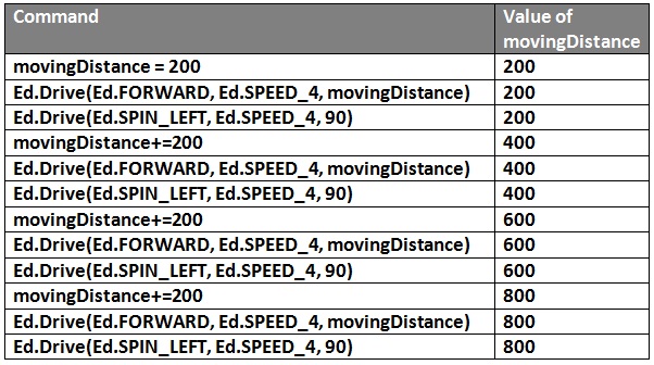
Tracing involves examining a piece of code and working out the values of the variables as we progress through the program's commands. Below we see a tracing of the program that we have just been discussing.
Figure 2: Tracing table
Tracing is normally done using pen and paper or else an online editable document such as Google Docs. It is used to trace the values of variables as program are being executed.
Since our above program has only one variable, our trace table has only two columns: commands, and value of variable. A program with more than one variable could have one column per variable.
Tracing Exercises
Tracing Exercise 1: In Coding Exercise 1 you have a variable movingDistance that holds the value of how far the robot is to travel at a particular point in its journey. The value stored in this variable varies as the program progresses. Using the image Tracing table above as an example create a tracing table for tracing the value of the variable movingDistance.
Tracing Exercise 2: Coding Exercise 2 is simply an extension of Coding Exercise 1. In the same manner extend Tracing Exercise 1 so that it tracks the values of the variable movingDistance as it reverses its journey through the second part of Coding Exercise 2.
"""The purpose of this program is to introduce a learner programmer to the conceptof variables. It builds on a previous program that the learner should be familiar with, i.e. a program that made the robot move around the perimeter of a square. In this case the program will not describe the perimeter of a square but instead will be achieved by creating a variable that will hold the value of theforward distance of the robot.At the beginning the variable is initialised to the value of the first forward move, then after the first move and turn of the robot the variable is thenincremented by 200 so that the next forward move will be 200cm longe than the previous move."""#initialise variable movingDistance to 300movingDistance = 300#Move forward by a distance of 200cm - since movingDistance has a value of 300Ed.Drive(Ed.FORWARD, Ed.SPEED_4, movingDistance)#Make an 90 degree turn leftEd.Drive(Ed.SPIN_LEFT, Ed.SPEED_4, 90)#Increment the value of movingDistance to 500movingDistance+=200#Move forward by a distance of 200cm - since movingDistance has a value of 500Ed.Drive(Ed.FORWARD, Ed.SPEED_4, movingDistance)Ed.Drive(Ed.SPIN_LEFT, Ed.SPEED_4, 90)#Increment the value of movingDistance to 700movingDistance+=200#Move forward by a distance of 200cm - since movingDistance has a value of 700Ed.Drive(Ed.FORWARD, Ed.SPEED_4, movingDistance)Ed.Drive(Ed.SPIN_LEFT, Ed.SPEED_4, 90)#Increment the value of movingDistance to 900movingDistance+=200#Move forward by a distance of 200cm - since movingDistance has a value of 900Ed.Drive(Ed.FORWARD, Ed.SPEED_4, movingDistance)Ed.Drive(Ed.SPIN_LEFT, Ed.SPEED_4, 90)movingDistance+=200
Commenting means writing lines into a program code that the compiler will ignore. This means that they won't affect the running of the program.
So why do we write comments? One reason is that we can describe in everyday English what the program is doing. This can be useful if the program is handed over to another programmer to maintain or alter. It can also be useful for the original programmer because if he or she comes back to it after a long time they may have forgotten the details of what the program did. In this case the comments should be helpful.
In Python there are two types of comments: multiline and single line comments. The multiline comment starts with triple quotation marks and also finishes with the same. This type of comment is useful when you with to write a long detailed comment. In our example above our multiline comment spans lines 1 to 13, where it describes in general terms the functionality of the program, what its goals are and how it relates to previous programs.
Single line comments begin with the hash symbol, "#". The line can be as long as the editor allows, but cannot go on to another line. If you wish to break it to a second line then that line must also begin with a hash.
The single line comments are used to describe individual lines of code or a group of related lines. For novice programmers it is a good way of helping the novice consolidate his or her knowledge of the concepts of the programme by having to describe the individual lines that make up the concepts.
Naturally an experienced programmer will not comment every single line, but instead will comment individual sections of the program. The novice however, should comment each line, especially when the program is relatively short.
Commenting Exercise 1: Using Listing 4 as an example, write line by line comment on Coding Exercise 1. You may also write a multiline comment at the beginning, describing in general what the program is doing. 2 to 3 lines of a comment is sufficient.
Commenting Exercise 2: Extend Commenting Exercise 1 to commenting on Coding Exercise 2. If you are adding multiline comments it is better to have a combined multiline at the start of the program as in Listing 4 than two short multiline comments.
In this page we looked at variables. They were initially introduced as being somewhat similar to their algebraic cousins. Initially this is a good way to introduce them if the novice programmers are already familiar with algebraic variables, as the cognitive load will be reduced. Although this will hold true for programming variables they differ from their algebraic relatives in some areas. The most obvious difference is that their names are longer than one letter, and the name may actually describe the data that is to be stored in the variable. The most important difference is that variables physically exist as reserved locations in a computer's memory when the program that contains them is running.
Novice programmers often hav misconceptions about variables:
Variables are simply pairing a name with a value. This is not the case. During the running of the program shown in Figure 2: Testing table, the value of the variable movingDistance starts at 200, then goes up to 400, then 600 and finally 800.
A variable can store any amount of values. Not true. Again the testing table in Figure 2 demonstrates this. In line 4 the value in movingDistance changes from 200 to 400. At this point the original value of 200 has disappeared and cannot be retrieved. Again at line 7 the value in movingDistance changes from 400 to 600. Once again the previous value of 400 is lost.
During the running of a program the value stored in a variable can change any number of times. One way of getting novice programmers to understand the different concepts of programming is to get them, usually using pen and paper or a Google Doc to follow a program line by line and determine what is the value of a variable at each stage of the processing. This is known as tracing.
Although not directly related to variables, commenting is another teaching method for helping novice programmers to comprehend a program. Commenting, however, is not a teaching technique that is to be abandoned once the programmers become more proficient in the art of programming. It is a very useful way of documenting large programs, so that subsequent maintenance of them can be easier.
The work requested here will contribute to your grade in AS91883 Create a computer program. As more concepts are studied the work on this assignment will be either extended, or else modified to incorporate facilities provided by the other concepts.
NCEA requirements
A computer program uses:
variables storing at least two types of data (e.g. numeric, text, Boolean)
sequence, selection and iteration control structures
input from a user, sensors or another external source
and one or more of:
data stored in collections (e.g. lists, arrays, dictionaries)
user-defined methods, functions or procedures.
This part of the assignment covers sequence and variables. Other programming concepts are to be covered in subsequent parts of the same assignment.
Brief
You are required to create a program to make the robot to perform at least four forward movements and turns. Each forward movement must be greater than the previous by a constant amount and the angle of each turning must be greater than its predecessor by a constant amount.
After performing its final move/turn the robot must retrace its steps using the same lengths and angle turns as its forward journey but in reverse order.
For planning your project you must use a sheet of paper or hard cardboard with a minimum size of A1. Using ruler, protractor and pencil you must plot the forward journey of the robot. (There is no need to plot the reverse journey since the robot will be retracing its journey backwards.) Also you must plan the journey so that it fits inside the sheet.
Once the physical plan is complete you must design an algorithm. Before writing the code it is advisable to test the algorithm using unplugged activities. Once no errors are discovered you may then use the algorithm to create a program to control the robot. Before testing the program on the robot you must first create a trace table to follow the values of the program variables. Use the tracing table example in Figure 2 as a model for this. Also use the coding exercises that you have created above, i.e. Coding Exercises 1 to 4. as reference models.