Python Programming

NCEA Compatibility

Module: as91906 Use complex programming techniques to develop a computer program

Requirements: reading from, or writing to, files or other persistent storage

Learninng Outcomes

On completion of this section you will know how to:

• Create a database
• Define and add a table to the same database
• Store processed data in the database
• Retrieve data from the database

Introduction

In the previous section we looked at storing data in text files. This technique is simple but the amount of processing available on the stored data is very limited and even that processing has to be individually coded.

Databases on the other hand allow us much greater scope for processing the stored data, especially if we are familiar with SQL. We can retrieve records based on a person’s name, the date of the transaction or any other criteria we wish. We can also update a number of records simultaneously or remove records that are no longer needed. Also it is easy to interface the database with other applications.

Creating a Database

In order to work with a database the first thing we must do is to actually create one. Listing 1 below shows us how to do that.

                            #C11 Create database.py
                            import sqlite3
                            connection =sqlite3.connect("Workers.db")
                            cursor=connection.cursor()
                            cursor.execute("create table workers(emplname text, hours real, rate real, gross real,tax real, net real)")
                            connection.commit()
                            cursor.close()
                    

Line 2 imports the module sqlite3. This is a module that comes with the Python system and it contains routines for processing a database.

Line 3 uses the connect() function from sqlite3 to create or open a database named “Workers.db”. Although it looks very different its function is quite similar to the command for opening a text file that we encountered in the previous chapter, i.e. myfile=open(“Workers.txt”,”a”). In both cases a text file or a database is opened if it already exists and is created if it does not exist. This, however, is where any similarities to text files end.

A database is a far more sophisticated data storage than a text file and opening it is not enough for storing data into it. To begin with we will have two pointers for working with the database, one for controlling the database itself and another for controlling its contents, which in our case means its tables.

The pointer for controlling the database itself is called the connection and at line 3 the variable storing it is also called connection.

The pointer for controlling the contents of the database is called the cursor and at line 4 a pointer to it is created, also called cursor.

As stated before processing the database is done by running SQL statements. In our case we use the execute() function of the cursor to run those SQL statements. We see an example of this in line 5 where we use the create table SQL statement to create a table named workers which has fields named emplname, hours, rate, gross, tax, SuperContribution and net. Apart from the first field, which is of type text, all the other fields are of type real, i.e. they can hold floating point numbers.

By the time line 5 is executed a table is defined for the database but may still be held in the computer’s memory instead of written to the database file itself. To ensure that it is written to the file we use the connection.commit() as shown in line 6.

As our table is already created, we don’t need our cursor any longer so we close it at line 7.

Adding Payroll Data to the Database

                        #C11 Payroll Dbase.py
                        
                        #Import relevant modules
                        import C9_Payroll_Module
                        import sqlite3
                        
                        #input section
                        strName = input("Enter employee's full name:  ")
                        floatHours = float(input("Enter value for hours:  "))
                        floatRate= float(input("Enter value for rate:  "))
                        
                        #processing section
                        floatGross = C9_Payroll_Module.calculateGross(floatHours, floatRate)
                        floatTax = C9_Payroll_Module.calculateTax(floatGross)
                        floatNet = C9_Payroll_Module.calculateNet(floatGross,floatTax)
                        
                        #output section
                        connection =sqlite3.connect("Workers.db")
                        cursor=connection.cursor()
                        strSQL="insert into workers values('"+strName+"', "+str(floatHours)+", "+str(floatRate)
                        strSQL+=", "+str(floatGross)+", "+str(floatTax)+", "+str(floatNet)+")"
                        print(strSQL)
                        cursor.execute(strSQL)
                        connection.commit()
                        cursor.close()
                    

Lines 1 to 15 of Listing 2 are identical to their equivalents in the two previous chapters and we shall therefore concentrate on the output section which spans lines 18 - 25.

Lines 18 and 19 open the database and establish a connection in almost the same way as in Listing 1. The only difference here is that since the database “Workers.db” was already existing, no new database was created – only the existing one was opened.

Next we have to create an SQL statement in order to store the payroll details in the table workers. The SQL statement is crated at lines 20 and 21.

Let us look at how the statement is created.

We shall first assume that during the input stage the user entered the following data: Tom Thumb for the employee’s name and 20, 30 respectively for the hours and rate. Thus, after processing is complete, the variables we wish to store in the database have values as shown in the table below.

The SQL statement must therefore look as follows:

insert into workers values('Tom Thumb', 20, 30.0, 600.0, 158.0, 442.0)

Line 20, by mixing string constants and the variables strName, floatHours and floatRate together creates the first part of the SQL statement, i.e.

insert into workers values('Tom Thumb', 20.0, 30.0

while line 21 adds the following to it:

, 600.0, 158.0, 442.0)

Thus the two together create a complete SQL statement.

Line 22 prints out the newly created SQL statement. This is purely for our reference only so we can double check that a properly structured statement was created at lines 20 and 21, and in a real life application would not normally occur.

Line 23 runs the SQL statement in the database which means creating a new record and adding the data shown in table 1 above to its fields.

Line 24 ensures that the data is written to the physical file on the disk and line 25 closes the cursor.

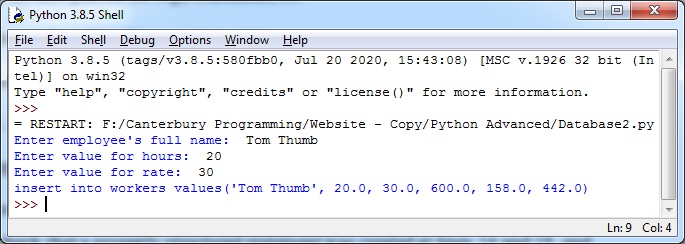
Figure 1 above shows a run-through of our application.

Reading Data from the Database

                       #C11 Read database.py
                        import sqlite3
                        connection =sqlite3.connect("Workers.db")
                        cursor=connection.cursor()
                        cursor.execute("SELECT * from workers")
                        result=cursor.fetchall()
                        for rec in result:
                            emplname, hours, rate, gross, tax, net=rec
                            print(emplname, hours, rate, gross, tax, net)
                        cursor.close()
                    

Listing 3 above is purely for reading the contents of the database, or more precisely the contents of the table workers within that database.

Lines 2, 3 and 4 work in the exact same way as their equivalents do in Listing 1 and Listing 2, so we shall leave them and concentrate on the rest of the code especially lines 5 to 9.

Line 5 runs an SQL query - Select * from workers - on the database. This is much shorter than any of the previous one and therefore needs an explanation. Firstly the keyword select means that we are reading data from the database not adding or modifying the data that is there. The ‘*’ means that we will read every field in the record. This means that the short SQL statement above is equivalent to Select emplname, hours, rate, gross, tax, net from workers. The outcome is that the system will read every field of every record in the database.

Line 6 calls the fetchall() function to retrieve the selected data and store it in the variable result. If the database table workers has four records in it result will have a list with four items in the list. Of course since each of the records in the database has seven fields in it, each one of the four items of our list is a list in its own right with seven items in it.

Lines 7 to 9 is a for loop. The loop variable rec starts with pointing to the first item, i.e. the first record in the list.

Line 8 reads the seven fields in rec and stores then in the variables emplname, hours, rate, gross, tax, and net.

Line 9 simply prints each of the above variables.

Lines 7 to 9 are repeated for every other record in rec and when all records are processed control goes to line 10 where the close() function closes the database connection.

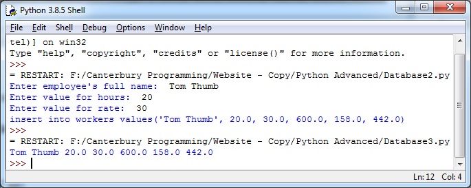
Fig 2 below shows the result of running this code.

Summary

Databases comprise a more flexible way of storing data as opposed to text files. As well as creating a database you must create a structured table inside the database in which to store your data. The table is created using the CREATE TABLE SQL statement.

Data is entered into the database using the INSERT INTO SQL statement. Data is retrieved from the database using the SELECT SQL statement.

Practice

Copy listing 1 into an editor and save it as a Python file. Next run it and check that a database is actually created.

Next copy Listing 2 into an editor then save and run it. Enter at least one record into the database.

Finally copy Listing 3 and save and run it like the others. It should display the results of the data you have just entered.

Exercise

• What module must you import in order to be able to create a database?
• State some of the differences between a database and a text file.
• Can you store data directly in a database?
• Through what medium do you get data from the compute into the database?
• How do you read data back from the database?

Revision

• What is the primary advantage of using a database over a text file?
  1. Easier syntax for storage
  2. Greater scope for processing stored data
  3. Requires no software libraries
  4. Unlimited storage capacity
• Which module is required to create and manage a SQLite database in Python?
  1. pandas
  2. sqlite3
  3. database
  4. sqlhandler
• What is the purpose of the cursor.execute() function in database operations?
  1. To close the database connection
  2. To write data to a text file
  3. To execute SQL commands
  4. To create backup files
• In Listing 1, what is the name of the created table?
  1. employees
  2. payroll
  3. workers
  4. jobs
• What SQL command is used to retrieve all fields from a table?
  1. INSERT INTO
  2. CREATE TABLE
  3. SELECT * FROM
  4. DELETE FROM
• What is the correct order of steps to add data to a database table?
  1. Open database → Insert data → Commit changes → Close cursor
  2. Insert data → Open database → Close cursor → Commit changes
  3. Commit changes → Open database → Insert data → Close cursor
  4. Open database → Close cursor → Insert data → Commit changes
• Which SQL statement is used to define a table in a database?
  1. SELECT
  2. INSERT INTO
  3. CREATE TABLE
  4. UPDATE
• What does the fetchall() function return when reading from a database?
  1. A single record as a dictionary
  2. A list of all records
  3. The structure of the database
  4. A count of rows in the database
• What happens if you run the sqlite3.connect("Workers.db") command and the file does not exist?
  1. An error is raised
  2. The database is automatically created
  3. The program terminates
  4. It returns a null connection
• What is the correct function to ensure changes to a database are saved to disk?
  1. cursor.save()
  2. connection.commit()
  3. database.write()
  4. save_changes()

Fill in the Blanks

• The Python module used to interact with SQLite databases is called _________.
• To ensure data is written to a database file after executing SQL statements, the function _________ is used.
• The SQL command used to create a new table in a database is _________.
• In Listing 1, the database file is named _________.
• The SQL command SELECT * FROM workers retrieves _________ from the workers table.
• The _________ function is used to fetch all the results of an SQL query in Python.
• A database table is defined with fields, each having a specific _________ type.
• The cursor object in Python is created using the _________ function of the connection object.
• In the database example, the field emplname stores the _________ of the employee.
• Databases offer more _________ for processing data compared to text files.

Assignment

Modify the assignment you created for Assignment Part 10 so that instead of storing data in a text file it will store it in a table within a database. This means that you will be dealing with three applications:

• A new application that creates a database and a table within it. This table will have to be structured so that it can accommodate all of the data required for sales processing. You can use listing 1 as a model for this application.
• Modify your existing application so that instead of storing data to a text file it will store it to the database created above. You can use Listing 2 as a model.
• A new application that will open the database and extract all of the data and then display them on the console. You can use Listing 3 as a model for this application.